Assessing the Complete Block Design

Prof Randi Garcia, SDS 290

2024-10-16

Announcements

SDS Presentation of the Major on Tuesday
HW 5 due Friday 10/18 11:59p
Exam 1 self-scheduled 10/25-10/27
Office hours (Bass 412)
- Friday: 3:00-4:00p
Where to get HW help
- Spinelli center tutoring Sun-Thurs 7-9p, Sabin-Reed 301. Nora Z, Cindy, and Sarah can help with 290.
- Post questions to hw5-questions Slack channel.

Agenda

MP1 data collection!
Complete Block design

MP1 data collection

Step 1:

If you’re approved:
- 20 minutes to go through the checklist.
- Paste anonymous survey link in the spreadsheet.
- If you’re ready, work on your homework!
If you’re NOT approved
- Use this time to work on your revisions.

Step 2:

25 min to participate in as many studies as you can!
- Note: see content notes
- Please only participate in audio studies if you have headphones

Inappropriate Insects

Modern zoos try to reproduce natural habitats in their exhibits as much as possible. They try to use appropriate plants, but these plants can be infested with inappropriate insects. Cycads (plants that look vaguely like palms) can be infected with mealybugs, and the zoo wishes to test three treatments: 1) water, 2) horticultural oil, and 3) fungal spores in water. Nine infested cycads are taken to the testing area. Three branches are randomly selected from each tree, and 3 cm by 3 cm patches are marked on each branch. The number of mealybugs on the patch is counted. The three treatments then get randomly assigned to the three branches for each tree. After three days the mealybugs are counted again. The change in number of mealybugs is computed (\(before-after\)).

Side-by-side lineplot

We add our blocking factor as color and also as group.

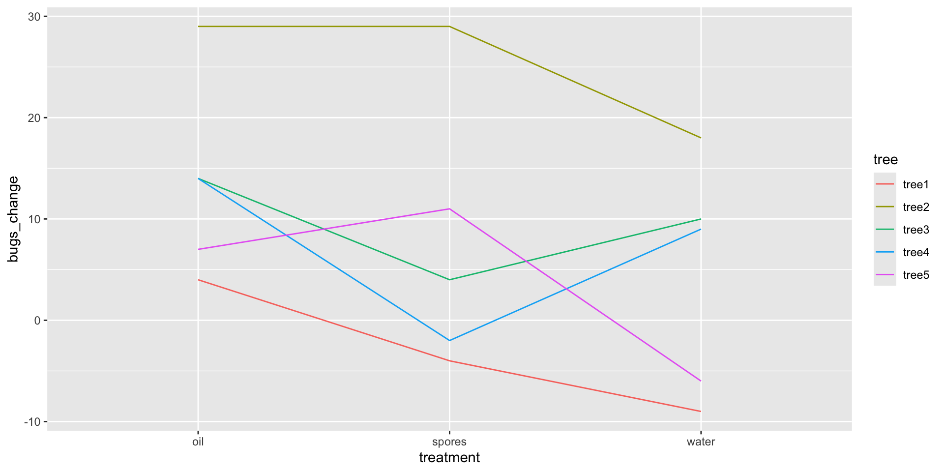
ggplot(mealybugs, aes(x = treatment, y = bugs_change, color = tree, group = tree)) + 
  geom_line()

We can see that Tree 2’s infestation was very responsive to the treatments whereas Tree 1’s was not.

Formal ANOVA for Complete Block Design

\[{y}_{ij}={\mu}+{\tau}_{i}+{\beta}_{j}+{e}_{ij}\]

Source	SS	df	MS	F
Treatment	\(\sum_{i=1}^{a}b(\bar{y}_{i.}-\bar{y}_{..})^{2}\)	\(a-1\)	\(\frac{{SS}_{T}}{{df}_{T}}\)	\(\frac{{MS}_{T}}{{MS}_{E}}\)
Blocks	\(\sum_{j=1}^{b}a(\bar{y}_{.j}-\bar{y}_{..})^{2}\)	\(b-1\)	\(\frac{{SS}_{B}}{{df}_{B}}\)	\(\frac{{MS}_{B}}{{MS}_{E}}\)
Error	\(\sum_{i=1}^{a}\sum_{j=1}^{b}({y}_{ij}-\bar{y}_{i.}-\bar{y}_{.j}+\bar{y}_{..})^{2}\)	\((a-1)(b-1)\)	\(\frac{{SS}_{E}}{{df}_{E}}\)

Data Analysis Structure

mealybugs

    tree treatment bugs_change
1  tree1     water          -9
2  tree1    spores          -4
3  tree1       oil           4
4  tree2     water          18
5  tree2    spores          29
6  tree2       oil          29
7  tree3     water          10
8  tree3    spores           4
9  tree3       oil          14
10 tree4     water           9
11 tree4    spores          -2
12 tree4       oil          14
13 tree5     water          -6
14 tree5    spores          11
15 tree5       oil           7

Formal ANOVA

mod <- lm(bugs_change ~ treatment + tree, data = mealybugs)

anova(mod)

Analysis of Variance Table

Response: bugs_change
          Df  Sum Sq Mean Sq F value   Pr(>F)   
treatment  2  218.13  109.07  2.9963 0.106846   
tree       4 1316.40  329.10  9.0412 0.004603 **
Residuals  8  291.20   36.40                    
---
Signif. codes:  0 '***' 0.001 '**' 0.01 '*' 0.05 '.' 0.1 ' ' 1

There are no statistically significant differences in the reduction in mealy bugs between the three treatment conditions, \(F(2, 8) = 3.00\), \(p = .107\). There are significant differences in the reduction in mealy bugs across trees, however, \(F(4, 8) = 9.04\), \(p = .005\). That is, some trees improved more than other trees.

Informal Analysis Structure

mealybugs_wide <- mealybugs %>%
  pivot_wider(names_from = treatment, values_from = bugs_change)

mealybugs_wide

# A tibble: 5 × 4
  tree  water spores   oil
  <chr> <dbl>  <dbl> <dbl>
1 tree1    -9     -4     4
2 tree2    18     29    29
3 tree3    10      4    14
4 tree4     9     -2    14
5 tree5    -6     11     7

How to check assumptions

C. Constant effects – think about whether it is reasonable.
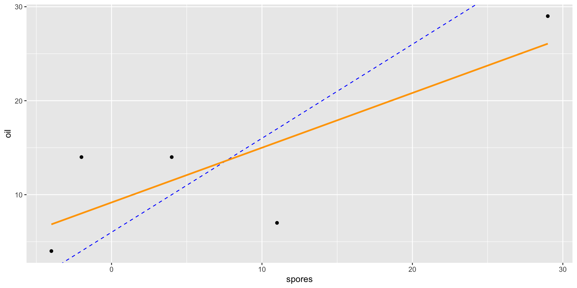
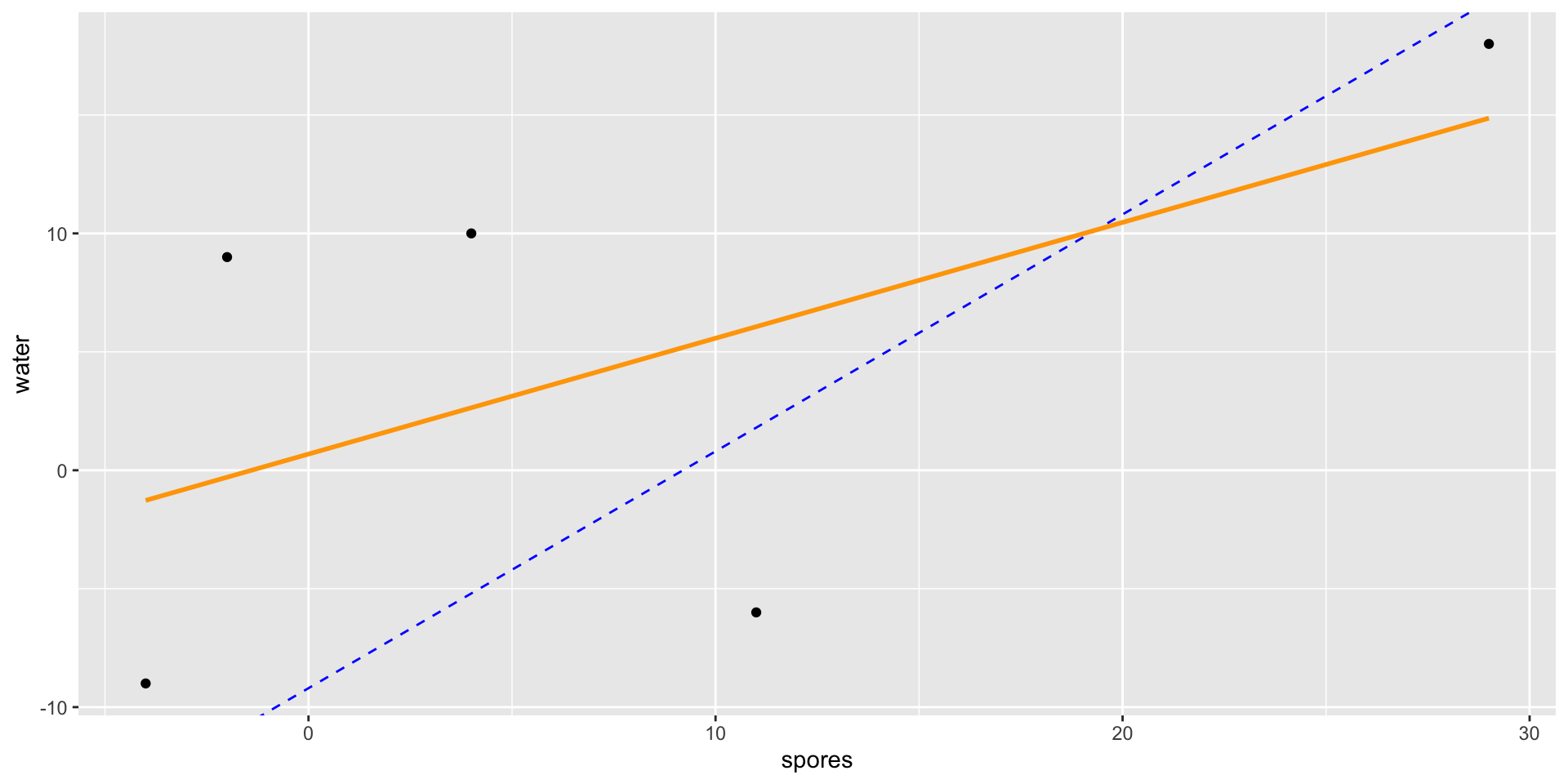
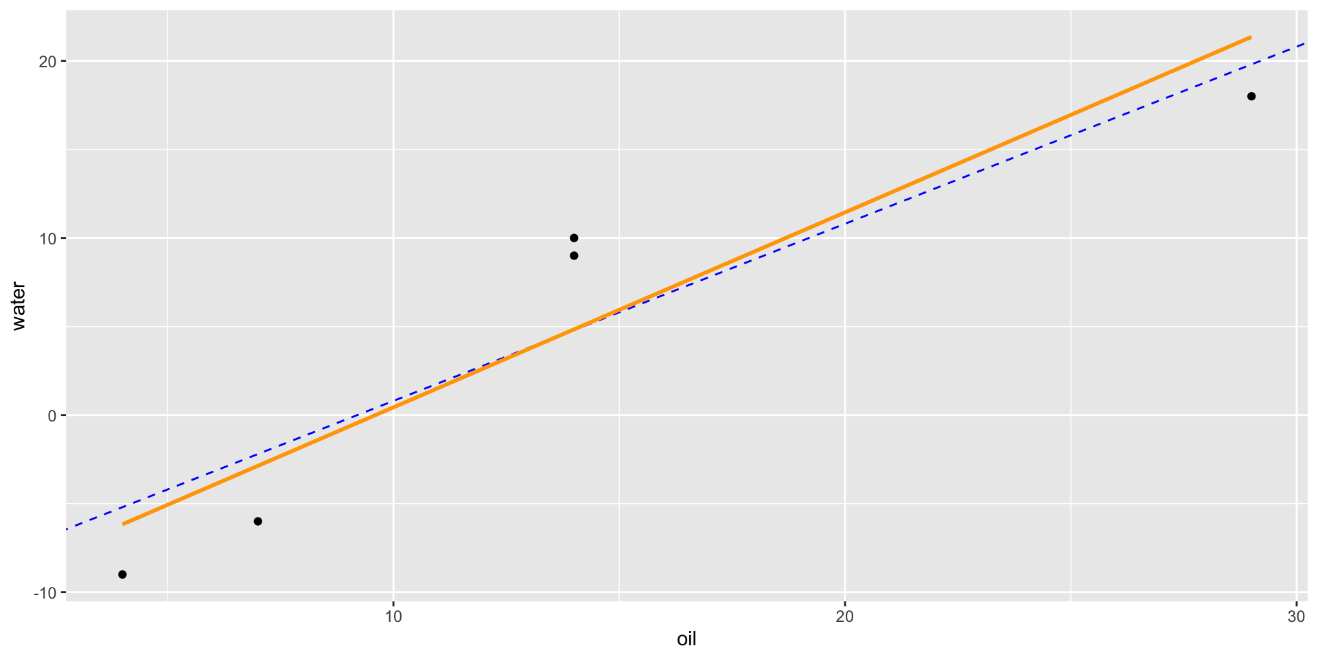
A. Additive effects – check Anscombe block plots.
S. Same standard deviations – is the biggest SD less than two times as large as the smallest? check residual versus fitted plot: does the plot thicken?
I. Independent residuals – think about whether it is reasonable.
N. Normally distributed residuals – construct a histogram or normal probability plot of residuals.
Z. Zero mean residuals – construct a histogram or normal probability plot of residuals.

Anscombe Block Plots

Scatterplots of two levels of the factor of interest.
Used for
- exploring the data, and
- assessing the additivity (A) condition.

Informal Analysis Structure

mealybugs_wide <- mealybugs %>%
  pivot_wider(names_from = treatment, values_from = bugs_change)

mealybugs_wide

# A tibble: 5 × 4
  tree  water spores   oil
  <chr> <dbl>  <dbl> <dbl>
1 tree1    -9     -4     4
2 tree2    18     29    29
3 tree3    10      4    14
4 tree4     9     -2    14
5 tree5    -6     11     7

Anscombe Block Plots

qplot(x = spores, y = oil, data = mealybugs_wide) +
  geom_abline(intercept = 13.6-7.6, slope = 1, color = "blue", linetype = 2) + 
  geom_smooth(method = "lm", se = 0, color = "orange")

Anscombe Block Plots

qplot(x = spores, y = water, data = mealybugs_wide) +
  geom_abline(intercept = 4.4 - 13.6, slope = 1, color = "blue", linetype = 2) + 
  geom_smooth(method = "lm", se = 0, color = "orange")

Anscombe Block Plots

qplot(x = oil, y = water, data = mealybugs_wide) +
  geom_abline(intercept = 4.4 - 13.6, slope = 1, color = "blue", linetype = 2) + 
  geom_smooth(method = "lm", se = 0, color = "orange")

Assessing S Condition

mealybugs %>%
  group_by(treatment) %>%
  summarize(m = mean(bugs_change),
            sd = sd(bugs_change))

# A tibble: 3 × 3
  treatment     m    sd
  <chr>     <dbl> <dbl>
1 oil        13.6  9.66
2 spores      7.6 13.3 
3 water       4.4 11.5

mealybugs %>%
  group_by(treatment) %>%
  summarize(m = mean(bugs_change),
            sd = sd(bugs_change)) %>%
  summarize(max(sd)/min(sd)) #calculating using min and max function

# A tibble: 1 × 1
  `max(sd)/min(sd)`
              <dbl>
1              1.38

Assessing S Condition

\[\hat{{y}}_{ij}={\mu}+{\tau}_{i}+{\beta}_{j}\]

Where \(\hat{{y}}_{ij}\) are the fitted values, that is, everything but the ticket at the end of the assembly line.

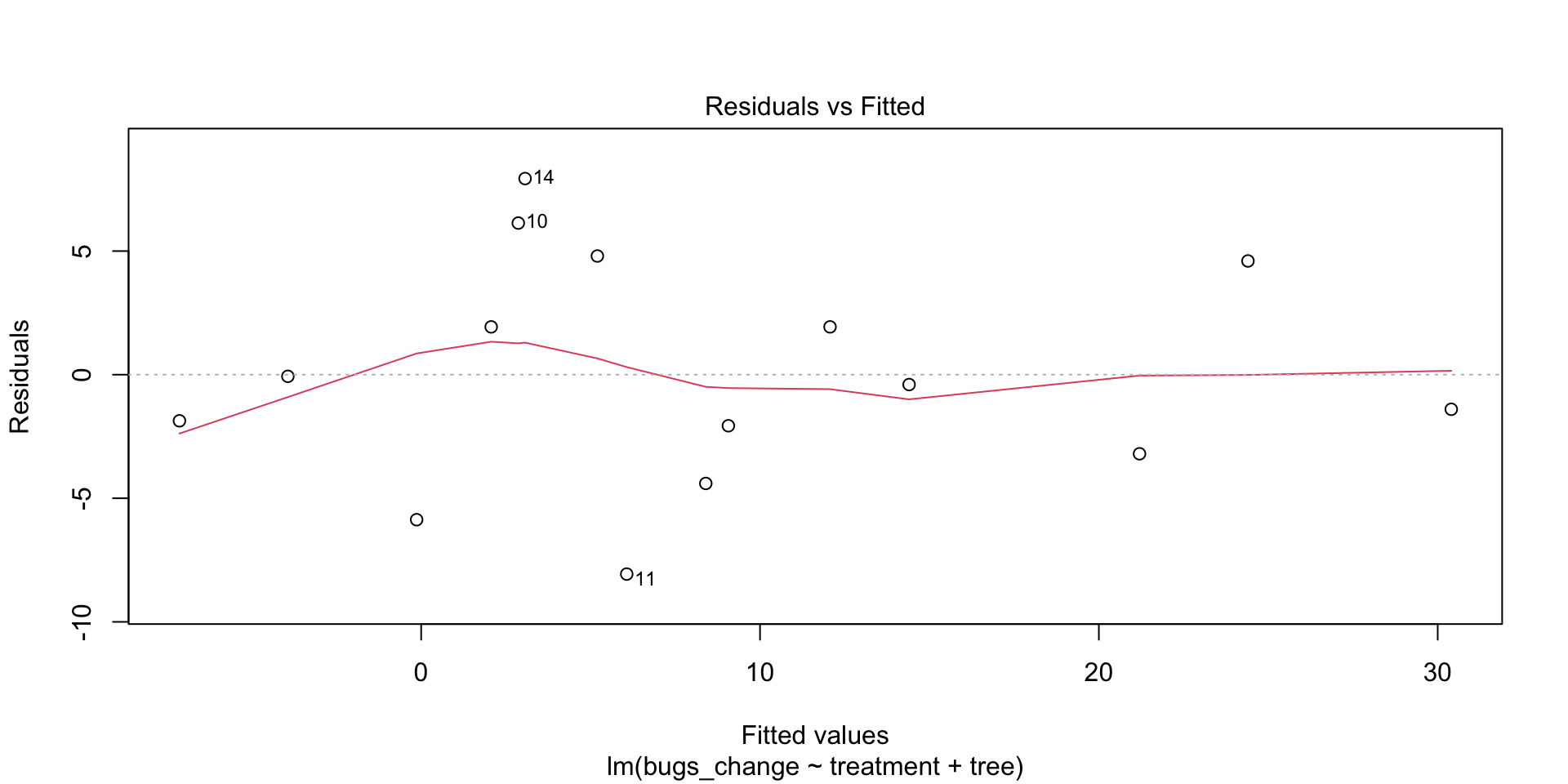
plot(mod, which = 1)

If the plot thickens, that is, has a patterning that looks like a funnel, then the S condition is not satisfied.

Assessing N Condition

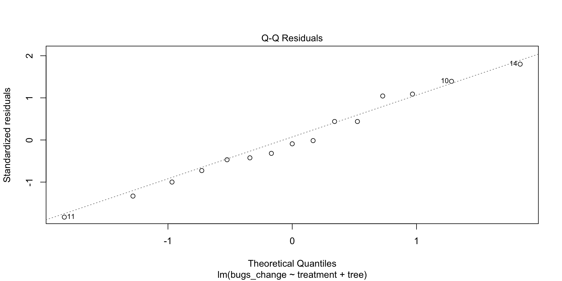
plot(mod, which = 2)

We’re looking for residuals to be on the line. If so, then we can say they are normally distributed.

Assessing the Z Condition

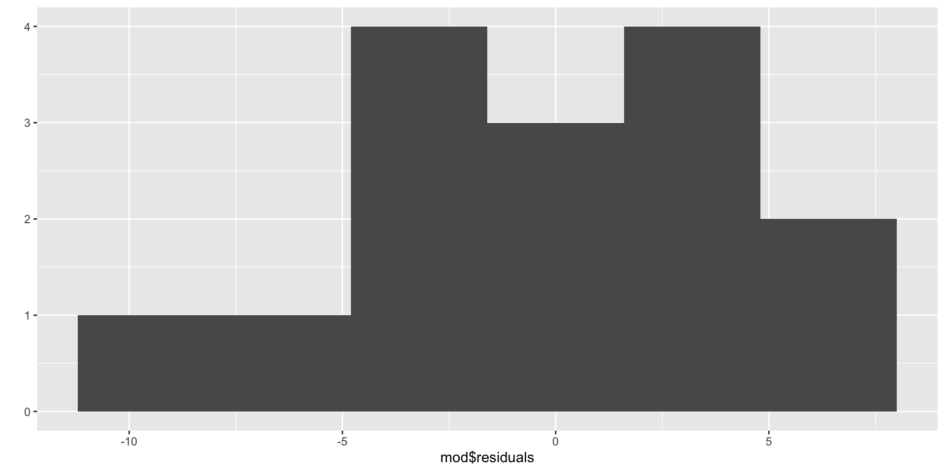
qplot(mod$residuals, bins = 6)

If the histogram centered at zero? Then the Z condition is satisfied.

Sleeping Shrews

Assess the CA-SINZ conditions for the SleepingShrews dataset from example 6.7b in your textbook.

library(Stat2Data)
data("SleepingShrews")

#You'll need the WIDE dataset for the Anscombe block plots
SleepingShrews_wide <- SleepingShrews %>%
  select(-ID) %>%
  pivot_wider(names_from = Phase, values_from = Rate)

Testing Condition for Sleeping Shrews Data

qplot(x = DSW, y = LSW, data = SleepingShrews_wide) +
  geom_abline(intercept = 2, slope = 1, color = "blue", linetype = 2) +   
  geom_smooth(method = "lm", se = 0, color = "orange") #A condition

qplot(x = DSW, y = REM, data = SleepingShrews_wide) +
  geom_abline(intercept = 2, slope = 1, color = "blue", linetype = 2) +   
  geom_smooth(method = "lm", se = 0, color = "orange") #A condition

qplot(x = LSW, y = REM, data = SleepingShrews_wide) +
  geom_abline(intercept = -2, slope = 1, color = "blue", linetype = 2) +   
  geom_smooth(method = "lm", se = 0, color = "orange") #A condition

SleepingShrews %>%
  group_by(Phase) %>%
  summarize(m = mean(Rate),
            sd = sd(Rate)) %>%
  summarize(max(sd)/min(sd)) #S condition

mod <- lm(Rate ~ Phase + Shrew, data = SleepingShrews)
plot(mod, which = 1) #S condition
plot(mod, which = 2) #N condition
qplot(mod$residuals, bins = 6) #N and Z conditions