# A tibble: 2 × 3
  arms_reduction num_responses   pct
  <fct>                  <int> <dbl>
1 against                  452 0.440
2 favor 576 0.560Inference for a single proportion
IMS, Ch. 16
Prof Randi Garcia
2026-03-23
Nuclear Arms Reduction Survey
A simple random sample of 1,028 US adults in March 2013 found that 56% support nuclear arms reduction.
- Do a majority of US adults support nuclear arms reduction?
Sample proportion (\(\widehat{p}\))
Response: arms_reduction (factor)
# A tibble: 1 × 1
   stat
  <dbl>
1 0.560- Note:
p_hatis a \(1 \times 1\)data.frame p_hat$statis the actual value
NHST Setup
- \(H_0: p = 0.5\)
- \(H_A: p \neq 0.5\)
- \(\alpha = 0.05\)
- How do we construct the null distribution?
Three methods for inference
- Use simulations
- parametric bootstrap (Ch. 16.1)
- Use probability theory
- today
- Use normal approximation
- mathematical model (Ch. 16.2)
Once we have the null distribution
What is the standard error?
What is the p-value?
What is our decision?
Method 1: Simulation
Parametric bootstrap (review)
- Draw samples from binomial distribution
Null distribution (simluated)
Null distribution (simulated, in black)
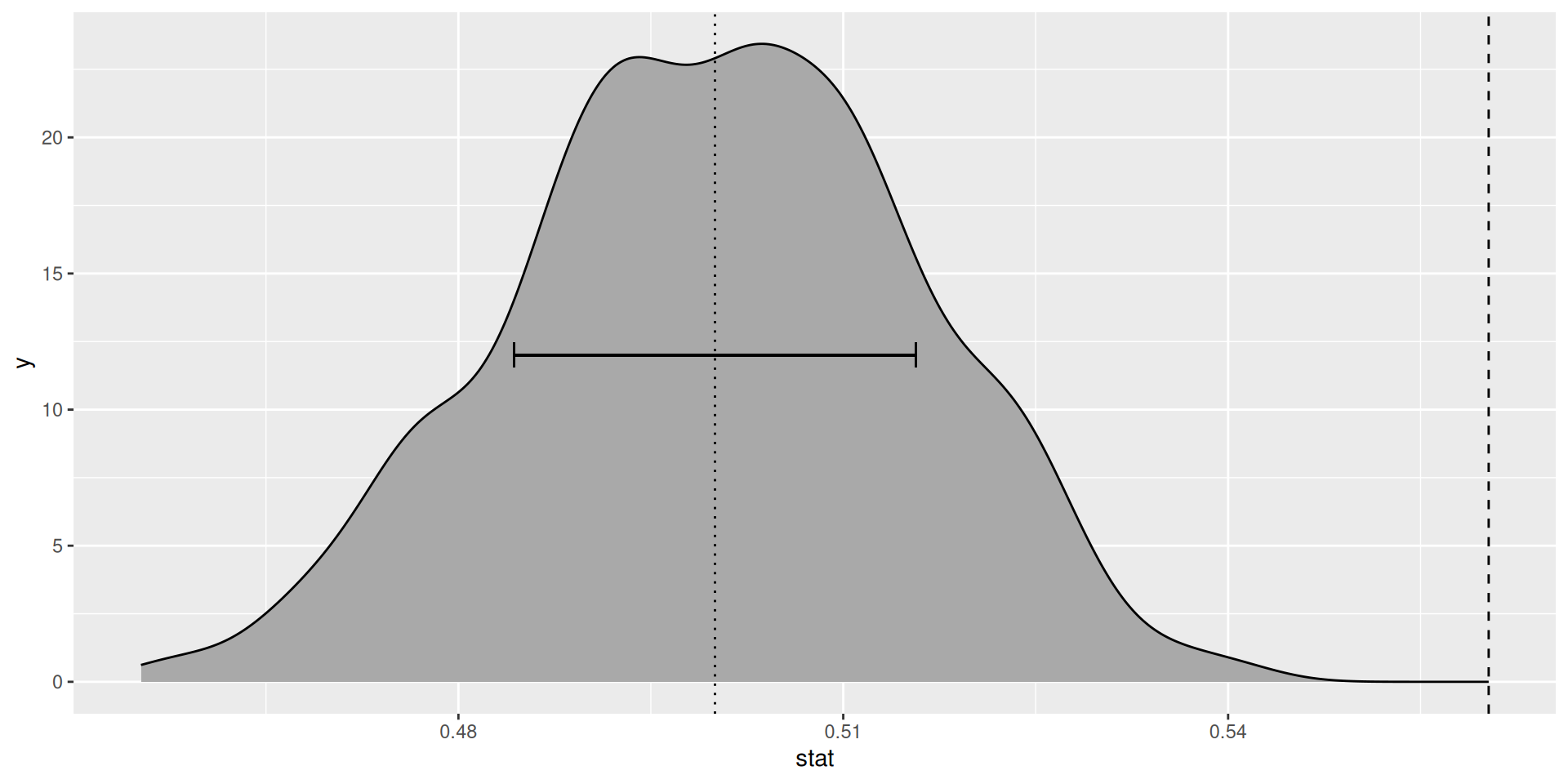
Standard error and p-value
- Standard error:
- p-value:
Your turn
- Does a majority support nuclear arms reduction?
Why simulate the null?
Pros:
- intuitive
- no math
- few assumptions
Cons:
- requires computer
- requires coding ability
- solution is approximate
- non-deterministic
- foreshadowing: Isn’t this equivalent to next method?
Method 2: Probability theory
Probability theory
- Compute exact null distribution
Let \(X \sim Bernoulli(p)\). Then,
\[ E[X] = p, Var[X] = p(1-p) \]
Let \(Y = X_1 + \cdots + X_n\). Then \(Y \sim Binom(n, p)\) and,
\[ E[Y] = np, Var[Y] = np(1-p) \]
Probability theory (cont’d)
\(Z = Y/n\) is a r.v. giving the mean of \(n\) draws from \(X\)!
Then,
\[ E[Z] = p \]
And,
\[ Var[Z] = \frac{1}{n^2} \cdot np(1-p) = \frac{p(1-p)}{n} \]
And, \(sd(Z) = \sqrt{\frac{p(1-p)}{n}}\) is the standard error!
Properties of null distribution
Same shape as binomial distribution curve
Has \(SE = \sqrt{\frac{p(1-p)}{n}}\)
se <- sqrt(p_0 * (1 - p_0) / n)

dbinom_p <- function (x, size, prob, log = FALSE) {
  1000 * dbinom(round(x * size), size, prob, log)
}

null_dist_2 <- null_dist +
  geom_function(
    fun = dbinom_p, color = "red",
    args = list(size = 1042, prob = p_0)
  ) +
  geom_errorbarh(
    aes(xmax = p_0 + se, xmin = p_0 - se, y = 10),
    color = "red"
  )
Null distribution (exact, in red)
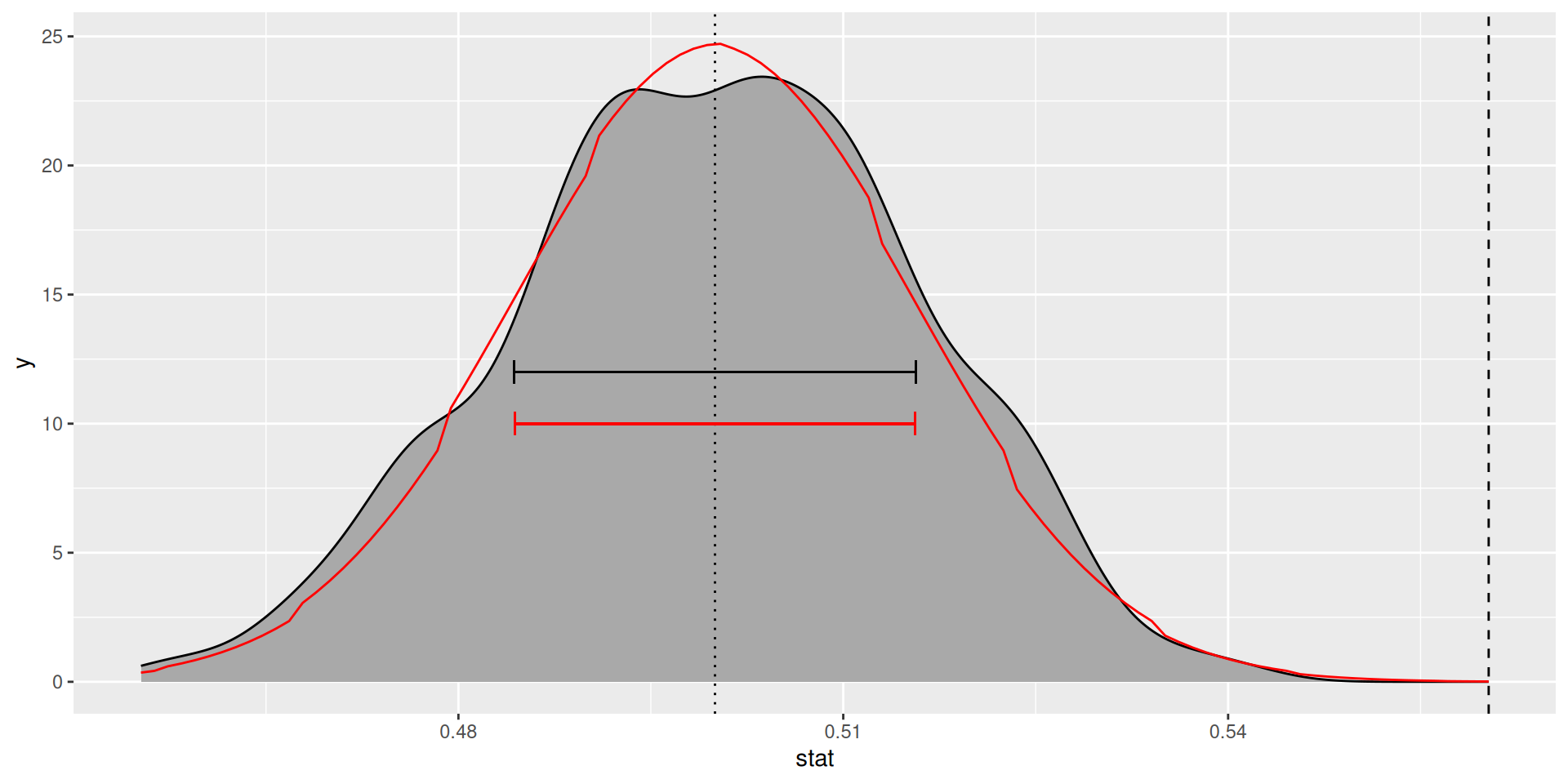
Standard error and p-value
- Standard error:
- p-value:
Your turn
Does a majority support nuclear arms reduction?
Compare the SE and p-value from the previous method. Are they meaningfully different?
Why compute the null?
Pros:
- correct answer
- deterministic
Cons:
- Had to do a bunch of math. Math wasn’t too bad in this case, but it gets much harder in other cases.
- only possible for simple situations
Method 3: Normal approximation
Normal approximation
By CLT, for \(n\) large enough, null distribution is approximately normal
If \(np_0 > 10\) and \(n(1-p_0) > 10\), then approximation is reasonably good
Use \(SE = \sqrt{\frac{p(1-p)}{n}}\) (from before)
- Now you know why!!
Null distribution (normal approx.)
Null distribution (approx., in blue)
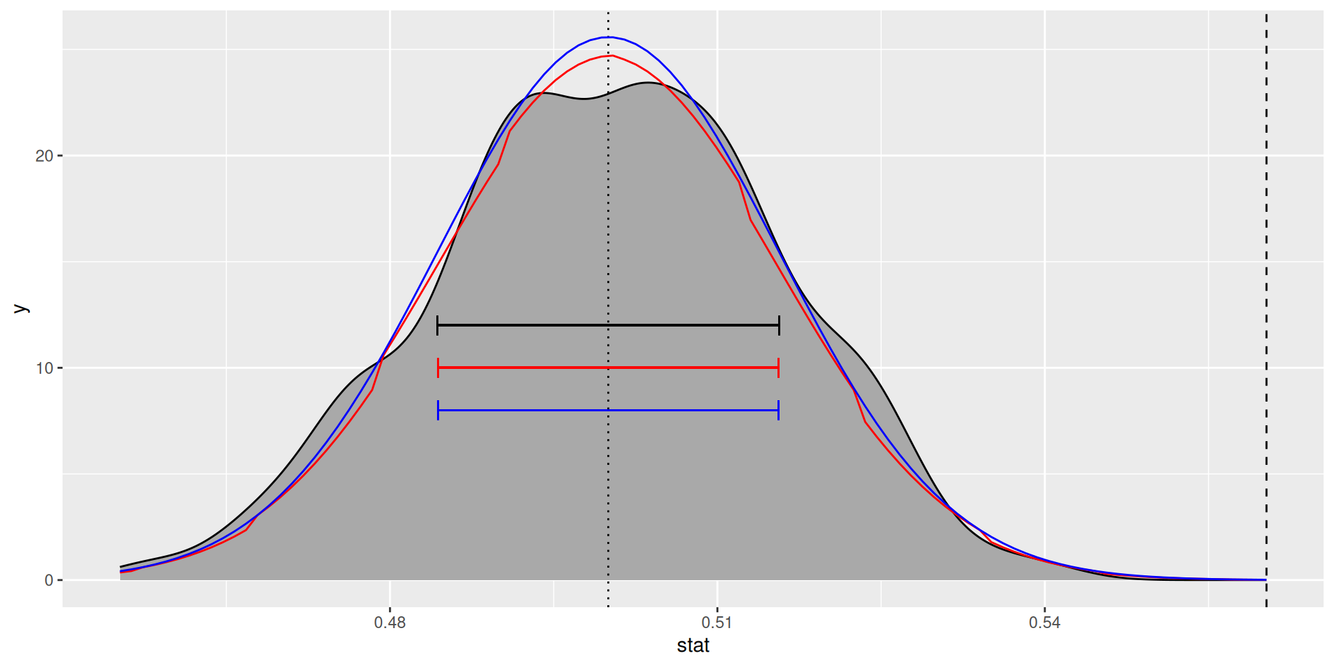
Standard error and p-value
- Standard error:
- p-value:
Z-scores
- Compute z-score:
- But,
- Is \(\widehat{p}\) in the rejection region?
Alternatively, using infer
Your turn
Does a majority support nuclear arms reduction?
Compare the SE and p-value from the previous method. Are they meaningfully different?
Why approximate the null?
Pros:
- provable approximation quality
- no computer required
- (kind of)
- deterministic
- widely-used
Cons:
Solution is approximate, and sometimes approximation is not great
SE formula comes out of nowhere
harder to connect to big ideas?
- Most common, well-understood method