| treatment | tree1 | tree2 | tree3 | tree4 | tree5 |
|---|---|---|---|---|---|
| oil | 4 | 29 | 14 | 14 | 7 |
| spores | -4 | 29 | 4 | -2 | 11 |
| water | -9 | 18 | 10 | 9 | -6 |
Exam 2 Review
Prof Randi Garcia, SDS 290
2024-12-02
Announcements
- HW9 due (tonight) Monday Dec 2 11:59p
- Exam 2 self-scheduled 12/6-12/8
- Or in class on Wednesday
- Office hours (Bass 412)
- Tuesday 10:30a - 11:30a
- Friday 3:00p - 4:00p
- Where to get HW9 help
- Post questions to #hw9-questions channel on Slack!
- Direct message me on Slack.
Exam 2
- Closed notes, closed book, closed internet
- 85 minute to complete the exam
- You can use your phone for a calculator
- Can have 1 single-sided notes page (“cheatsheet”).
- You do not need to turn it in with your exam.
Design Names
One-Way Design
- If the factor is a true experimental factor
- One-Way Randomized Design or
Design Names
Block design or Two-Way Additive Model
- There is one factor of interest and one nuisance factor (the blocking factor).
- If the factor of interest is experimental
- Randomized Block Design
- If every block gets every treatment
- Complete Block Design
Design Names
Two-Way Factorial Design
- If the factors of interest are experimental
- Randomized Two-Way Factorial
- There is no blocking in this design
Design Names
Split-Plot Design
- There is blocking in this design.
- There is (at least) one between-blocks factor
- There is (at least) one within-blocks factor
Design Principal: Blocking
- Blocking is using a factor that is not of research interest
- But there may be differences across blocks on the response variable
- A “block” is a level of a blocking factor
- We use blocking to improve precision/statistical power of our factor of interest
Three Ways to Block
- Sort units into similar groups
- Subdivide larger chunks of material into sets of smaller pieces
- Reuse subjects or material in each of several times slots
Complete Block Design
- Experimental material are separated into groups (or reused) to create similar units
- Then each unit within a block is then is assigned one level of the factor of interest
- “Complete Block” means that every block x treatment combination is tested
More Design Terminology
- The two factors Trees and Treatment are crossed. This means that we collect data on all combinations of Trees and Treatment. A cell is a particular combination.
- Main effect refers to the effect for a single factor. For a block design there are two sets of main effects, for blocks and for treatments (e.g., Trees and Treatment).
- The two sets of main effects are called additive if each treatment adds or subtracts the same amount to the response variable for all blocks.
- A factor of interest is Treatment, which is directly related to the goal of the study. A nuisance factor is Trees which is included as a factor only because it is a source of variation and its inclusion will reduce the sum of squares for error (residuals).
Inappropriate Insects
Draw the factor diagram.
Formal ANOVA for Complete Block Design
\[{y}_{ijk}={\mu}+{\tau}_{i}+{\beta}_{j}+{e}_{ijk}\]
| Source | SS | df | MS | F |
|---|---|---|---|---|
| Treatment | \(\sum_{i=1}^{a}b(\bar{y}_{i.}-\bar{y}_{..})^{2}\) | \(a-1\) | \(\frac{{SS}_{T}}{{df}_{T}}\) | \(\frac{{MS}_{T}}{{MS}_{E}}\) |
| Blocks | \(\sum_{j=1}^{b}a(\bar{y}_{.j}-\bar{y}_{..})^{2}\) | \(b-1\) | \(\frac{{SS}_{B}}{{df}_{B}}\) | \(\frac{{MS}_{B}}{{MS}_{E}}\) |
| Error | \(\sum_{i=1}^{a}\sum_{j=1}^{b}({y}_{ij}-\bar{y}_{i.}-\bar{y}_{.j}+\bar{y}_{..})^{2}\) | \((a-1)(b-1)\) | \(\frac{{SS}_{E}}{{df}_{E}}\) |
Formal ANOVA
Analysis of Variance Table

Response: bugs_change
          Df  Sum Sq Mean Sq F value   Pr(>F)
treatment  2  218.13  109.07  2.9963 0.106846
tree       4 1316.40  329.10  9.0412 0.004603 **
Residuals  8  291.20   36.40
---
Signif. codes:  0 '***' 0.001 '**' 0.01 '*' 0.05 '.' 0.1 ' ' 1
There are no statistically significant differences in the reduction in mealy bugs between the three treatment conditions, \(F(2, 8) = 3.00\), \(p = .107\). There are significant differences in the reduction in mealy bugs across trees, however, \(F(4, 8) = 9.04\), \(p = .005\). That is, some trees improved more than other trees.
How to check assumptions
C. Constant effects – think about whether it is reasonable.
A. Additive effects – check Anscombe block plots.
S. Same standard deviations – is the biggest SD less than two times as large as the smallest? check residual versus fitted plot: does the plot thicken?
I. Independent residuals – think about whether it is reasonable.
N. Normally distributed residuals – construct a histogram or normal probability plot of residuals.
Z. Zero mean residuals – construct a histogram or normal probability plot of residuals.
Anscombe Block Plots
- Scatterplots of two levels of the factor of interest.
- Used for
- exploring the data, and
- assessing the additivity (A) condition.
Informal Analysis Structure
Scatterplots
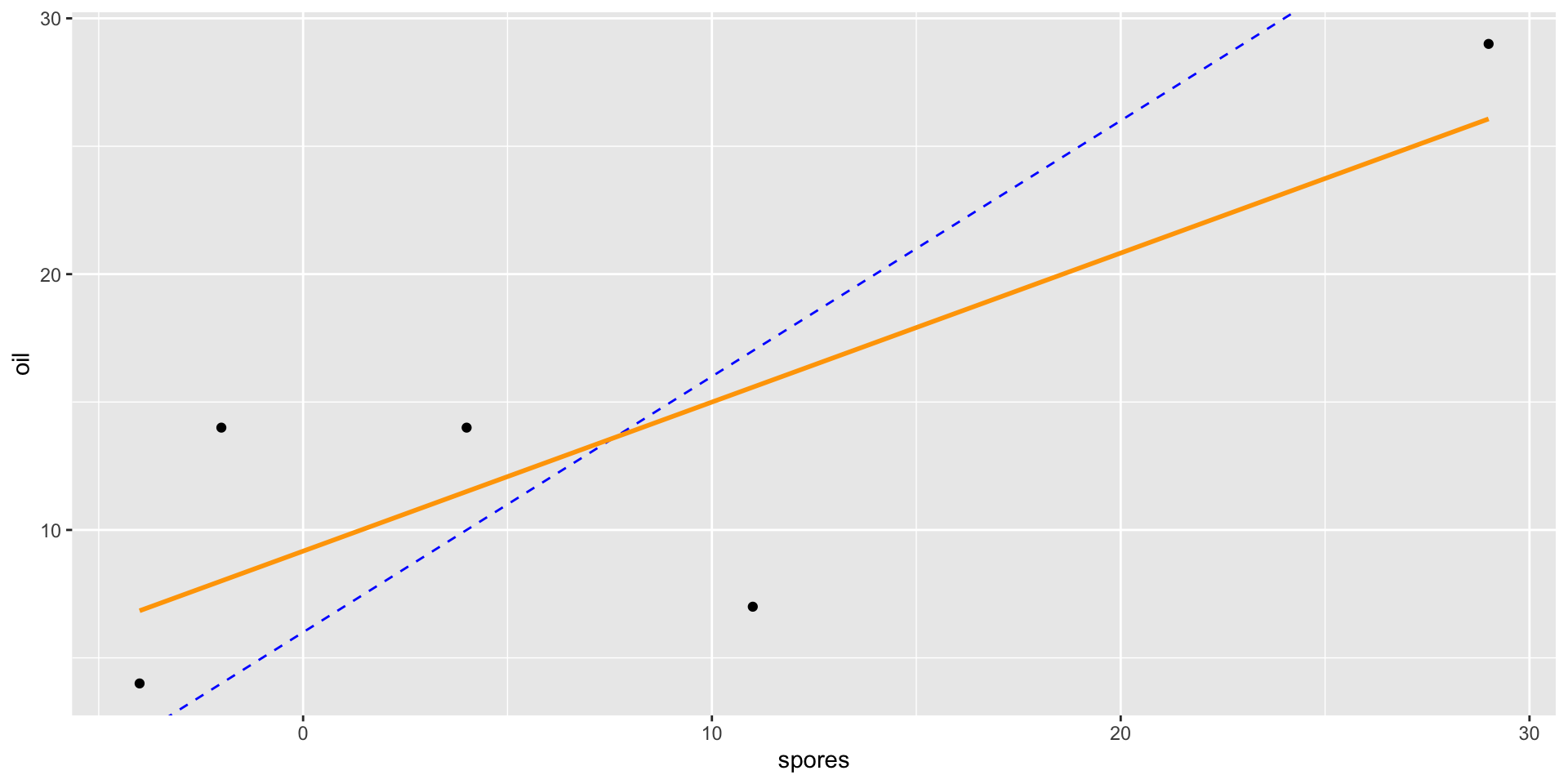
Scatterplots
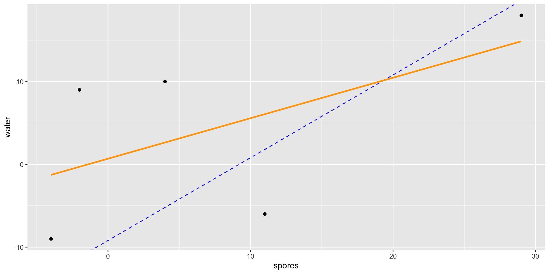
Scatterplots
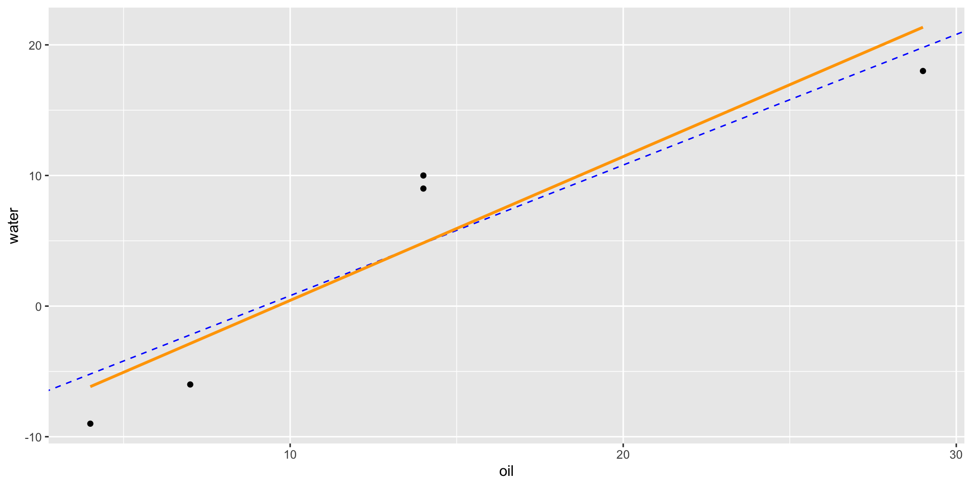
Two-Way Factorial Design Factor Diagram

- Draw the factor diagram
Research Questions in a Two-Way Factorial Design
- Does treatment A have an effect on the response variable?
- Is there a main effect of factor A?
- Does treatment B have an effect on the response variable?
- Is there a main effect of factor B?
- Does being in a specific combination of treatments have an effect over and above the additive effects of treatment A and B alone?
- Is there an interaction between factor A and factor B?
ANOVA Source Table for Two-Way Factorial
\[{y}_{ijk}={\mu}+{\alpha}_{i}+{\beta}_{j}+{\alpha\beta}_{ij}+{e}_{ijk}\]
| Source | SS | df | MS | F |
|---|---|---|---|---|
| Treatment A | \(\sum_{i=1}^{a}bn(\bar{y}_{i..}-\bar{y}_{…})^{2}\) | \(a-1\) | \(\frac{{SS}_{A}}{{df}_{A}}\) | \(\frac{{MS}_{A}}{{MS}_{E}}\) |
| Treatment B | \(\sum_{j=1}^{b}an(\bar{y}_{.j.}-\bar{y}_{…})^{2}\) | \(b-1\) | \(\frac{{SS}_{B}}{{df}_{B}}\) | \(\frac{{MS}_{B}}{{MS}_{E}}\) |
| Interaction AB | \(n\sum_{i=1}^{a}\sum_{j=1}^{b}(\bar{y}_{ij.}-\bar{y}_{i..}-\bar{y}_{.j.}+\bar{y}_{…})^{2}\) | \((a-1)(b-1)\) | \(\frac{{SS}_{AB}}{{df}_{AB}}\) | \(\frac{{MS}_{AB}}{{MS}_{E}}\) |
| Error | \(\sum_{i=1}^{a}\sum_{j=1}^{b}\sum_{k=1}^{n}({y}_{ijk}-\bar{y}_{ij.})^{2}\) | \(ab(n-1)\) | \(\frac{{SS}_{E}}{{df}_{E}}\) |
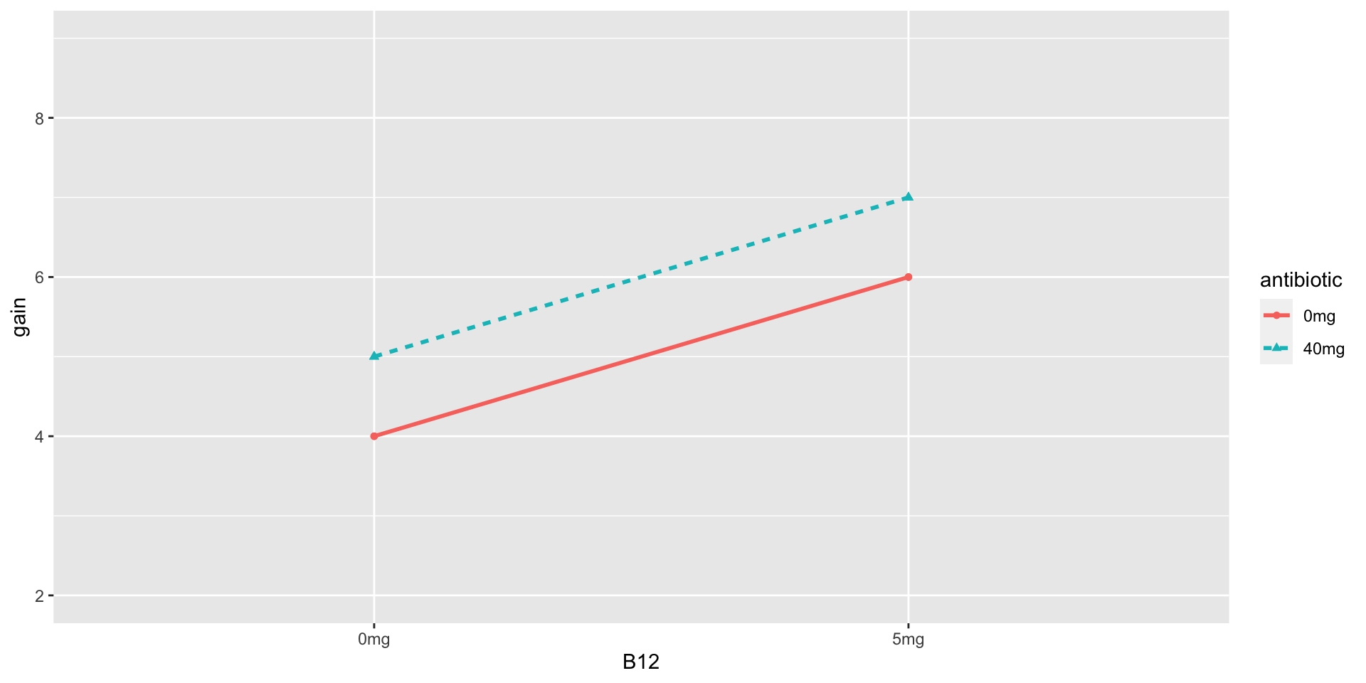
Interaction Graphs
For each of the following interaction graphs, answer the following questions with YES or NO.
- Is there a main effect of B12?
- Is there a main effect of antibiotics?
- Is there an interaction between B12 and antibiotics?
Practice 1
Confidence intervals and effect sizes
- If the interaction is significant
- Calculate CIs and effect sizes for sets of conditional averages (also called “simple effects”)
- For example, for the 0mg antibiotics condition, what’s the effect size for B12
- If the interaction is NOT significant
- Calculate CIs and effect sizes for sets of marginal averages (also called “main effects”)
- For example, what is the effect size for B12 overall?
Conditional Averages and Marginal Averages

- The numbers in blue are Marginal Averages
- The numbers in green are Conditional Averages
Confidence Intervals and Effect Sizes
Confidence Intervals
\[(\bar{y_i}-\bar{y_j}) \pm t^*\cdot SD \sqrt{1/n_i+1/n_j}\]
Effect size
\[D_{ij} = \frac{(\bar{y_i}-\bar{y_j})}{SD}\]
- Where \(SD = \sqrt{MSE}\)
Example: Walking Babies
Example: Walking Babies
So we fail to meet the condition of equal variances? (The S condition)
Levene’s Test
The biggest SD not more than 2 times as large as the smallest SD is only a rule of thumb.
Levene’s test is an ANOVA to test the null hypothesis:
\[H_0 = \sigma^2_1=\sigma^2_2=\sigma^2_3=\sigma^2_4\] \[H_A= not\:all\:variances\:are\:equal\]
Levene’s Test in R
Levene's Test for Homogeneity of Variance (center = median)
      Df F value Pr(>F)
group  3  0.3082 0.8191
      20
Using Levene’s Test for homogeneity of variance, we fail to reject the null hypothesis, that is we fail to find evidence that the S condition is not met, \(F(3, 20)=0.31\), \(p = .819\). We can proceed as if this condition is met.
Levene’s Test for Factorial Data
Let’s try it for the PigFeed data.
Levene's Test for Homogeneity of Variance (center = median)
      Df F value Pr(>F)
group  3  1.8089 0.2235
       8
Using Levene’s Test for homogeneity of variance, we fail to reject the null hypothesis, that is we fail to find evidence that the S condition is not met, \(F(3, 8)=1.81\), \(p = .224\). We can proceed as if this condition is met.
Multiple Tests
Fisher’s LSD
Bonferroni Correction
Tukey’s HSD
  Tukey multiple comparisons of means
    95% family-wise confidence level

Fit: aov(formula = Days ~ Diet, data = Leafhoppers)

$Diet
                 diff        lwr     upr     p adj
Fructose-Control  0.2 -0.9148496 1.31485 0.8805808
Glucose-Control   0.8 -0.3148496 1.91485 0.1337642
Sucrose-Control   1.8  0.6851504 2.91485 0.0095276
Glucose-Fructose  0.6 -0.5148496 1.71485 0.2677272
Sucrose-Fructose  1.6  0.4851504 2.71485 0.0145912
Sucrose-Glucose   1.0 -0.1148496 2.11485 0.0703156
Split-Plot Design
If you suspect a design in a split-plot design, you should be able to answer the following questions:
- What are the whole plots, that is, what is the nuisance factor?
- What is the between-blocks factor? Is it observational or experimental?
- What is the within-blocks factor? Is it observational or experimental?
Formal ANOVA for the Split-Plot Design
\[{y}_{ijk}={\mu}+{\alpha}_{i}+{\beta}_{j(i)}+{\gamma}_{k}+({\alpha\gamma})_{ik}+{e}_{ijk}\]
- \({\mu}\) is the benchmark
- \({\alpha}_{i}\) effect of level i of the between-blocks factor, \(i\) from \(1\) to \(a\)
- \({\beta}_{j(i)}\) effect of block \(j\) (for level \(i\) of the between block factor), \(j\) from \(1\) to \(n\)
- \({\gamma}_{k}\) effect of level \(k\) of the within-block factor, \(k\) from \(1\) to \(t\)
- \(({\alpha\gamma})_{ik}\) interaction effect for level \(i\) of the between-blocks factor with level \(k\) of the within-blocks factor
ANOVA Source Table for the Split-Plot Design
| Source | SS | df | MS | F |
|---|---|---|---|---|
| Between | \(t\frac{N}{a}\sum_{i=1}^{a}(\bar{y}_{i..}-\bar{y}_{...})^{2}\) | \(a-1\) | \(\frac{{SS}_{A}}{{df}_{A}}\) | \(\frac{{MS}_{A}}{{MS}_{B}}\) |
| Blocks | \(t\sum_{i=1}^{a}\sum_{j=1}^{n}(\bar{y}_{ij.}-\bar{y}_{i..})^{2}\) | \(N-a\) | \(\frac{{SS}_{B}}{{df}_{B}}\) | \(\frac{{MS}_{B}}{{MS}_{E}}\) |
| Within | \(Na\sum_{k=1}^{K}(\bar{y}_{..k}-\bar{y}_{...})^{2}\) | \(t-1\) | \(\frac{{SS}_{T}}{{df}_{T}}\) | \(\frac{{MS}_{T}}{{MS}_{E}}\) |
| Interaction | \(\sum_{i=1}^{a}\sum_{k=1}^{t}\frac{N}{a}(\bar{y}_{i.k}-\bar{y}_{i..}-\bar{y}_{..k}+\bar{y}_{...})^{2}\) | \((a-1)(t-1)\) | \(\frac{{SS}_{AT}}{{df}_{AT}}\) | \(\frac{{MS}_{AT}}{{MS}_{E}}\) |
| Error | \(\sum_{i=1}^{a}\sum_{j=1}^{N}\sum_{k=1}^{t}({y}_{ijk}-\bar{y}_{i.k}-\bar{y}_{.j.}-\bar{y}_{..k}+\bar{y}_{i..})^{2}\) | \((N-a)(t-1)\) | \(\frac{{SS}_{E}}{{df}_{E}}\) |
Piglets
Design: Two-Way Factorial Design
It seems natural to think that adding the right vitamins to a pig’s diet might produce fatter pigs faster. You’ve decided to study the effects of B12 in two doses (0mg and 5mg). But pigs have bacteria living in their intestines that might prevent the uptake of vitamins, so you decided to give antibiotics to the pigs in one of two doses (0mg or 40 mg). You design your experiment in such a way that 3 piglets are randomly assigned to each of the 4 treatment conditions. You measure their weight every day, and take each pig’s average daily weight gain as your final number recorded.
Albino laboratory rats
Design: Complete Block Design
Male albino laboratory rats are used routinely in many kinds of experiments. This experiment was designed to determine the requirements for protein in their food. Specifically, the experiment is interested in testing five levels of protein (8.68, 12, 15, 18, and 21% of diet). Baby rats were separated into ten groups of 5 to form groups of approximately the same weight. The 5 rats in each group were randomly assigned to each of the 5 conditions. Body weight and food consumption were measured twice weekly, and the average daily weight gain over 21 days was recorded.
Blood concentration
Design: Complete Block Design
This experiment is interested in the blood concentration of a drug after it has been administered. The concentration will start at zero, then go up, and back down as it is metabolized. This curve may differ depending on the form of the drug (a solution, a tablet, or a capsule). We will use three subjects, and each subject will be given the drug three times, once for each method. The area under the time-concentration curve is recorded for each subject after each method of drug delivery.
Paper Helicopters
Design: Two-Way Factorial Design
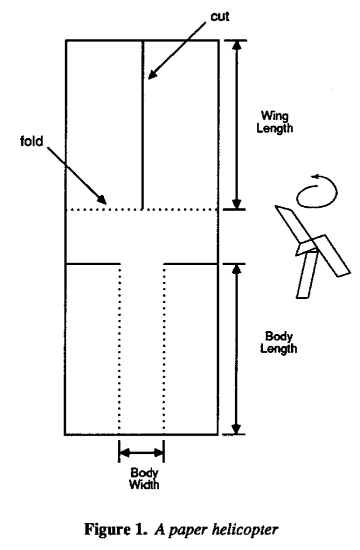
Paper helicopters can be cut from one half of an 8.5 by 11 sheet of paper. We can conduct an experiment by dropping helicopters from a fixed height and clocking the time it takes to drop. We can vary wing length: 4.25 in, 4.0 in, 3.75 in, and 3.5 in, as well as body width: 3.25 in, 3.75 in, 4.0 in, and 4.25 in. We’ll make 32 planes and randomly assign them to the 16 combinations.
Parks and Recreation
Design: One-Way Design
Deputy director of the Pawnee Parks and Rec department, Leslie Knope, needs to know how resistant different vegetative types are to trampling so that the number of visitors can be controlled in sensitive areas. Twenty lanes of a park are established, each .5 m wide and 1.5 m long. These twenty lanes are randomly assigned to five treatments: 0, 25, 75, 200, or 500 walking passes. Each pass consists of a 70-kg individual wearing boots, walking in a natural gait. One year after trampling, the average height of the vegetation along the lanes are measured.
Crabgrass
Design: Three-Way Factorial Design
The purpose of this experiment was to study the way one species of crabgrass competed with itself and with another species for nitrogen (N), phosphorus (P), and potassium (K). Bunches of crabgrass were planted in vermiculite, in 16 Styrofoam cups; after the seeds head sprouted, the plants were thinned to 20 plants per cup. Each of the 16 cups were randomly assigned to get one of 8 nutrient combinations added to its vermiculite. For example, yes-nitrogen/no-phosphorus/yes-potassium. The response is mean dry weight per plant, in milligrams.
Osomoregulation
Design: Split-plot Design
- Blocking factor: Worms
- Between-blocks factors: Water concentration; Species
- Within-blocks factor: Time
Worms that live at the mouth of a river must deal with varying concentrations of salt. Osomoregulating worms are able to maintain relatively constant concentration of salt in the body. An experiment wanted to test the effects of mixtures of salt water on two species of worms: Nereis virens (N) and Goldfingia gouldii (G). Eighteen worms of each species were weighted, then randomly assigned in equal numbers to one of three conditions. Six worms of each kind were placed in 100% sea water, 67% sea water, or 33% sea water. The worms were then weighted after 30, 60, and 90 minutes, then placed in 100% sea water and weighted one last time 30 minutes later. The response was body weight as percentage of initial body weight.
Creepy Animals
Design: Split-plot Design
- Blocking factor: Students
- Between-blocks factors: Animal
- Within-blocks factor: Posture (scary/submissive)
The effects of exposure to images of different domestic animal species in either aggressive or submissive postures on mood was tested with a split-plot/repeated measures design. Using a computer to randomize, participants were randomly assigned to either view images of dogs or images of cats. All participants saw both an aggressive animal and a submissive animal, and their moods were assessed via self-report after each image. The order of presentation (aggressive then submission, or submissive then aggressive) was randomized to control for order effects.