Two-Way Factorial Designs

Prof Randi Garcia, SDS 290

2024-10-28

Announcements

• Mini-Project 1 Technical Report due on Friday 11:59p on Moodle
• Office hours
  • Tuesday 10:30a - 11:30a
  • Friday 3:00p - 4:00p
• Where to get MP1 help
  • Office hours
  • Post questions to #mini-project1 channel on Slack!
  • Direct message me on Slack.

Agenda

2. MP1 data processing
3. Review blocking
   1. Assessing conditions in block designs
4. Two-Way Factorial Design

MP1 data analysis plan

Basic analysis plan…

1. I will download the data and clean it.
2. I will make a box plot to visualize the differences between groups.
3. I will calculate descriptive statistics and check the S assumption. Check for sample sizes in each condition.
4. If my N condition appears violated from the boxplots and/or my S condition is violated from the descriptive statistics I will try a log transformation if that seems like the obvious choice, or I will make a diagnostic plot by plotting log(sd) versus log(m).
5. If I decided to do a data transformation I will re-plot and re-test my conditions.
6. I will then run the one-way ANOVA model and state my conclusions based on appropriate statistics.
7. I will test or think about the rest of my ANOVA conditions.
8. I will then test pairwise comparisons using the Fisher’s LSD method.
9. I will also calculate effect sizes for these differences, confidence intervals, and the overall \(R^2\).
10. I will write up all of my analyses clearly in words and proofread before I submit my report!

Formal ANOVA for Complete Block Design

\[{y}_{ij}={\mu}+{\tau}_{i}+{\beta}_{j}+{e}_{ij}\]

Source	SS	df	MS	F
Treatment	\(\sum_{i=1}^{a}b(\bar{y}_{i.}-\bar{y}_{..})^{2}\)	\(a-1\)	\(\frac{{SS}_{T}}{{df}_{T}}\)	\(\frac{{MS}_{T}}{{MS}_{E}}\)
Blocks	\(\sum_{j=1}^{b}a(\bar{y}_{.j}-\bar{y}_{..})^{2}\)	\(b-1\)	\(\frac{{SS}_{B}}{{df}_{B}}\)	\(\frac{{MS}_{B}}{{MS}_{E}}\)
Error	\(\sum_{i=1}^{a}\sum_{j=1}^{b}({y}_{ij}-\bar{y}_{i.}-\bar{y}_{.j}+\bar{y}_{..})^{2}\)	\((a-1)(b-1)\)	\(\frac{{SS}_{E}}{{df}_{E}}\)

Data Analysis Structure

mealybugs

    tree treatment bugs_change
1  tree1     water          -9
2  tree1    spores          -4
3  tree1       oil           4
4  tree2     water          18
5  tree2    spores          29
6  tree2       oil          29
7  tree3     water          10
8  tree3    spores           4
9  tree3       oil          14
10 tree4     water           9
11 tree4    spores          -2
12 tree4       oil          14
13 tree5     water          -6
14 tree5    spores          11
15 tree5       oil           7

Formal ANOVA

mod <- lm(bugs_change ~ treatment + tree, data = mealybugs)

anova(mod)

Analysis of Variance Table

Response: bugs_change
          Df  Sum Sq Mean Sq F value   Pr(>F)   
treatment  2  218.13  109.07  2.9963 0.106846   
tree       4 1316.40  329.10  9.0412 0.004603 **
Residuals  8  291.20   36.40                    
---
Signif. codes:  0 '***' 0.001 '**' 0.01 '*' 0.05 '.' 0.1 ' ' 1

There are no statistically significant differences in the reduction in mealy bugs between the three treatment conditions, \(F(2, 8) = 3.00\), \(p = .107\). There are significant differences in the reduction in mealy bugs across trees, however, \(F(4, 8) = 9.04\), \(p = .005\). That is, some trees improved more than other trees.

How to check assumptions

• C. Constant effects – think about whether it is reasonable.

• A. Additive effects – check Anscombe block plots.

• S. Same standard deviations – is the biggest SD less than two times as large as the smallest? check residual versus fitted plot: does the plot thicken?

• I. Independent residuals – think about whether it is reasonable.

• N. Normally distributed residuals – construct a histogram or normal probability plot of residuals.

• Z. Zero mean residuals – construct a histogram or normal probability plot of residuals.

Anscombe Block Plots

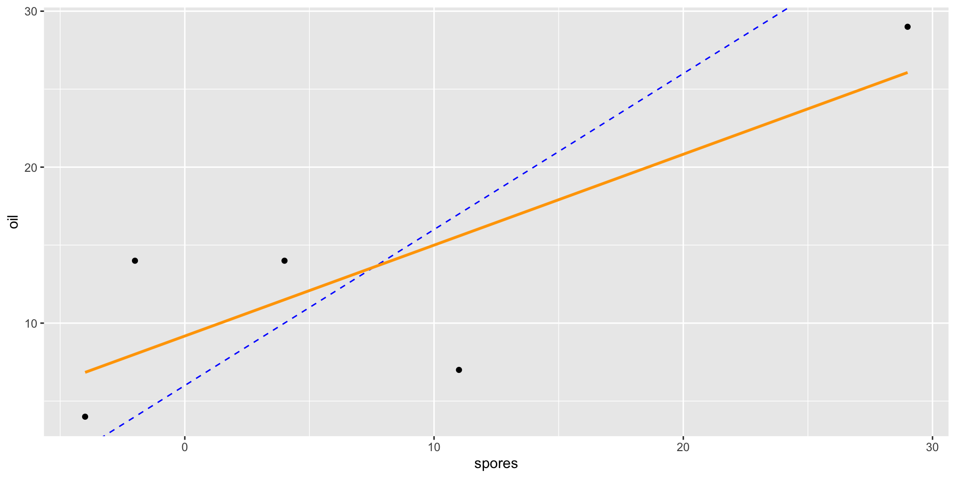
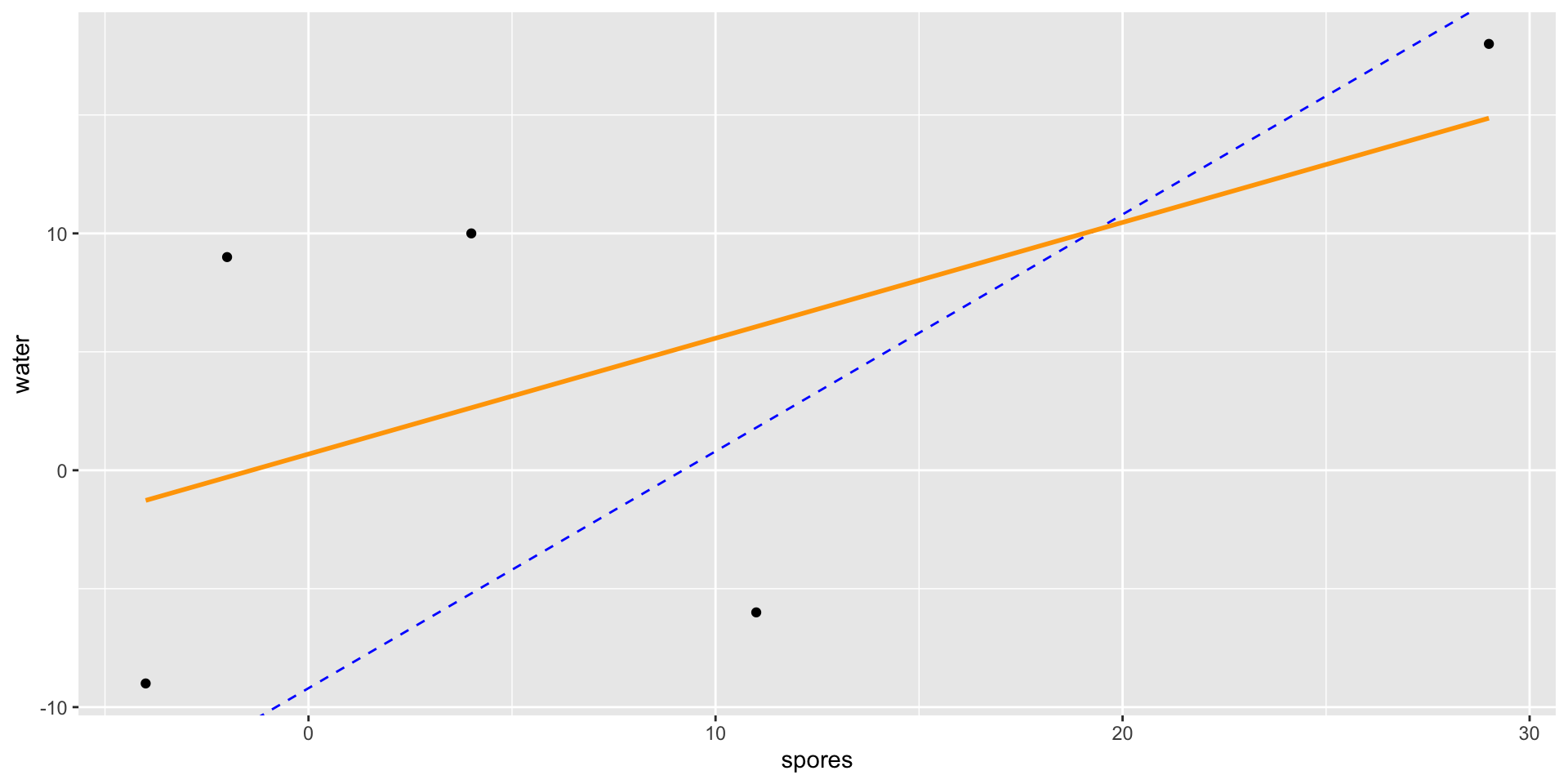
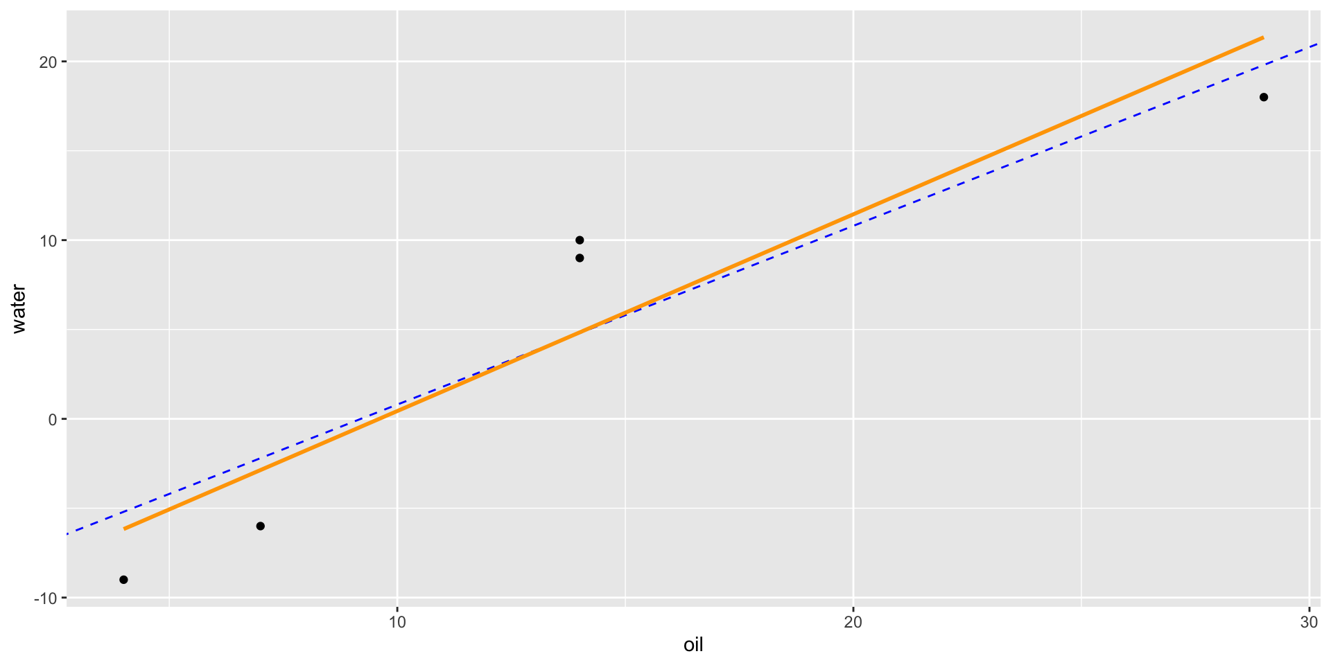
• Scatterplots of two levels of the factor of interest.
• Used for
  • exploring the data, and
  • assessing the additivity (A) condition.

Informal Analysis Structure

mealybugs_wide <- mealybugs %>%
  pivot_wider(names_from = treatment, values_from = bugs_change)

mealybugs_wide

# A tibble: 5 × 4
  tree  water spores   oil
  <chr> <dbl>  <dbl> <dbl>
1 tree1    -9     -4     4
2 tree2    18     29    29
3 tree3    10      4    14
4 tree4     9     -2    14
5 tree5    -6     11     7

Anscombe Block Plots

qplot(x = spores, y = oil, data = mealybugs_wide) +
  geom_abline(intercept = 13.6-7.6, slope = 1, color = "blue", linetype = 2) + 
  geom_smooth(method = "lm", se = 0, color = "orange")

Anscombe Block Plots

qplot(x = spores, y = water, data = mealybugs_wide) +
  geom_abline(intercept = 4.4 - 13.6, slope = 1, color = "blue", linetype = 2) + 
  geom_smooth(method = "lm", se = 0, color = "orange")

Anscombe Block Plots

qplot(x = oil, y = water, data = mealybugs_wide) +
  geom_abline(intercept = 4.4 - 13.6, slope = 1, color = "blue", linetype = 2) + 
  geom_smooth(method = "lm", se = 0, color = "orange")

Assessing S Condition

mealybugs %>%
  group_by(treatment) %>%
  summarize(m = mean(bugs_change),
            sd = sd(bugs_change))

# A tibble: 3 × 3
  treatment     m    sd
  <chr>     <dbl> <dbl>
1 oil        13.6  9.66
2 spores      7.6 13.3 
3 water       4.4 11.5 

mealybugs %>%
  group_by(treatment) %>%
  summarize(m = mean(bugs_change),
            sd = sd(bugs_change)) %>%
  summarize(max(sd)/min(sd)) #calculating using min and max function

# A tibble: 1 × 1
  `max(sd)/min(sd)`
              <dbl>
1              1.38

Assessing S Condition

Residual versus fitted plot

• Looking for no apparent pattern.
• Constant variance across fitted values.

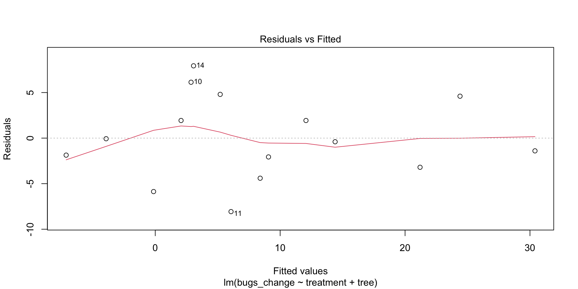
plot(mod, which = 1)

Assessing N Condition

Normal qq plot

• Looking for lining up of residuals on the straight line.

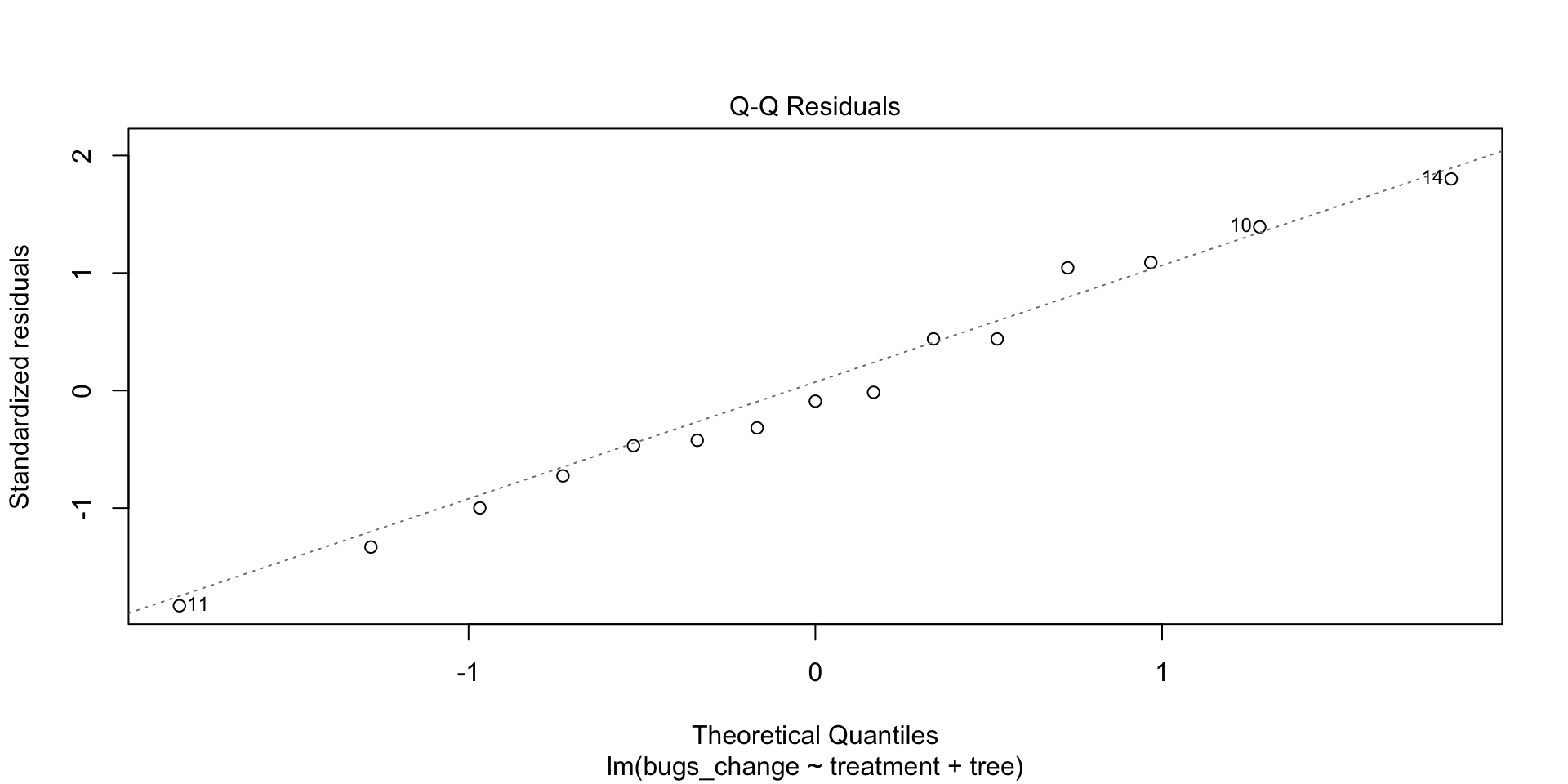
plot(mod, which = 2)