Multiple Comparisons

Prof Randi Garcia, SDS 290

2024-09-30

Announcements

HW4 due on Friday
Office hours (Bass 412)
- Tomorrow (tue) 10:30-11:30a
- Friday office hours cancelled
Where to get HW help
- Spinelli center tutoring Sun-Thurs 7-9p, Sabin-Reed 301. Nora Z, Cindy, and Sarah can help with 290.
- Post questions to hw4-questions Slack channel.

Agenda

Review
- CI and Effect sizes
Multiple Comparisons
MP1 topics time
- (More) Introduction to Qualtrics

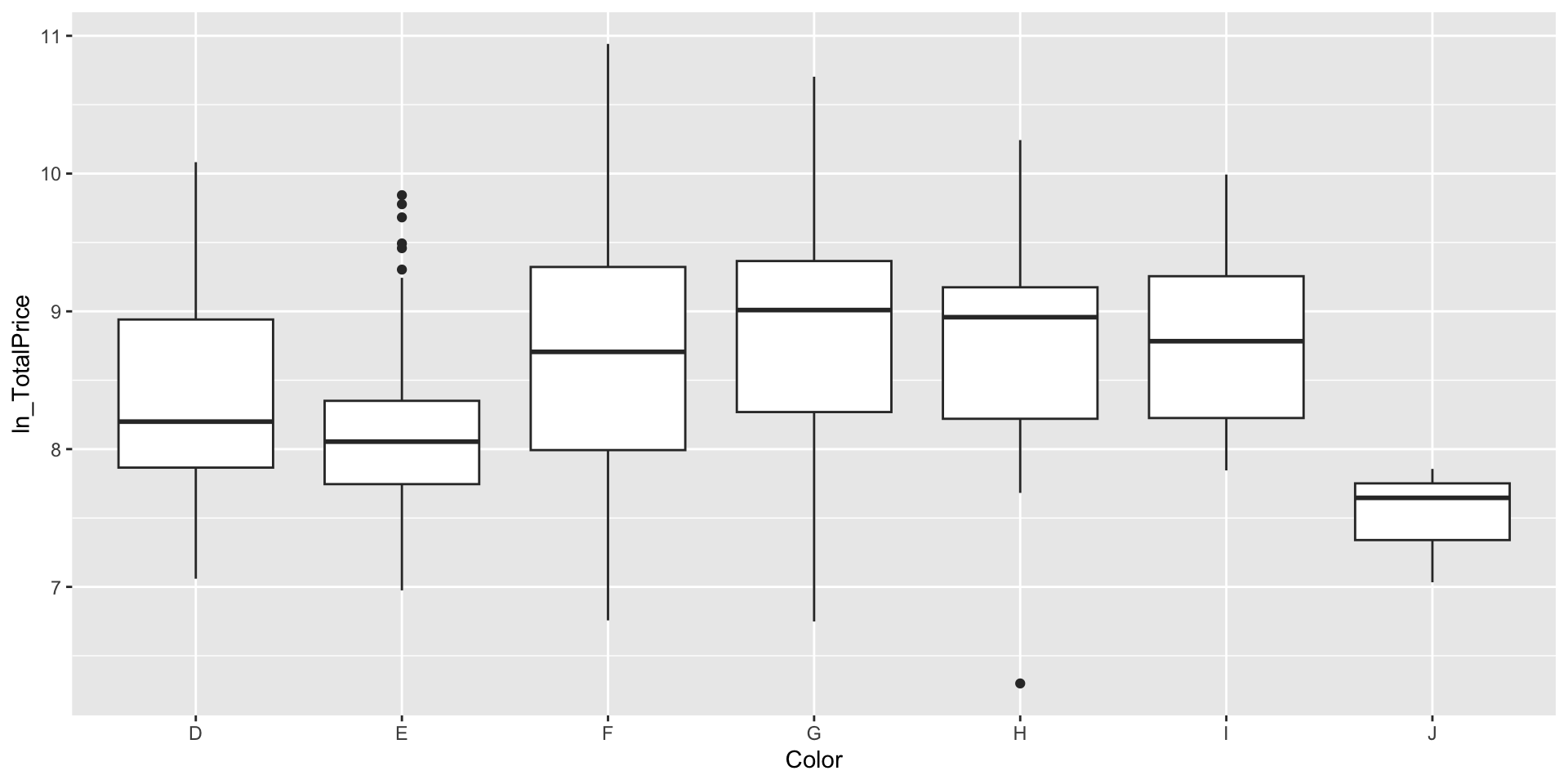
Diamond Price by Color

ggplot(Diamonds, aes(x = Color, y = ln_TotalPrice)) +
  geom_boxplot()

Descriptive statistics

We’ll need this later!

ds <- Diamonds %>%
  group_by(Color) %>%
  summarise(n = n(),
            m = mean(ln_TotalPrice),
            sd = sd(ln_TotalPrice))

ANOVA for Diamonds

modDia <- lm(ln_TotalPrice ~ Color, data = Diamonds)
anova(modDia)

Analysis of Variance Table

Response: ln_TotalPrice
           Df  Sum Sq Mean Sq F value    Pr(>F)    
Color       6  29.946  4.9909  7.3713 1.972e-07 ***
Residuals 344 232.913  0.6771                      
---
Signif. codes:  0 '***' 0.001 '**' 0.01 '*' 0.05 '.' 0.1 ' ' 1

There are statistically significant differences in log price of diamonds across colors \(F(6, 344) = 7.37\), \(p < .001\).

But what else do we want to know??

Effect Sizes and Confidence Intervals

The p-value for our F-ratio only tells us if effects are detectable.
- Answers the question: IS there an effect?
Practical significance is different from statistical significance.
- Need to answer the question: How big is IT?
Which values in ANOVA do we want to construct confidence intervals for (or calculate an effect size for)?

Some options:

A specific group mean.
How far away a specific condition is from the grand average (the treatment effect).
Pairwise group differences: How far away a specific condition is from another condition.
How far away a specific condition (or set of conditions) is(are) from a(nother) set of conditions.
Additional effect size option: The overall variance explained by a factor of interest.

CI for Pairwise Group Differences

\[(\bar{y_i}-\bar{y_j}) \pm t^*\cdot SD \sqrt{1/n_i+1/n_j}\]

Diamonds example: For difference between G (near colorless) and F (colorless)

MSE = 0.6771 #from our ANOVA source table
df_E = 344 #from our ANOVA source table
t <- qt(.975, df_E) #for 95% CI

n_g = filter(ds, Color == "G")$n #sample size for G
n_f = filter(ds, Color == "F")$n #sample size for F

mean_g <- filter(ds, Color == "G")$m #mean for G
mean_f <- filter(ds, Color == "F")$m #mean for F

#Confidence interval
UL <- (mean_g-mean_f) + t*sqrt(MSE)*sqrt(1/n_g+1/n_f) #upper limit
LL <- (mean_g-mean_f) - t*sqrt(MSE)*sqrt(1/n_g+1/n_f) #lower limit

LL

[1] -0.0168944

UL

[1] 0.4753144

We are 95% confident that the true mean difference in (log) price between near colorless and colorless diamonds is between -0.02 and 0.48. (There is no evidence of a difference between mean prices for colorless and near colorless diamonds.)

Effect Size

Effect Size (D)

\[D_{ij} = \frac{(\bar{y_i}-\bar{y_j})}{SD}\]

Where again \(SD = \sqrt{MSE}\)

D = (mean_g-mean_f)/sqrt(MSE)
D

[1] 0.2785525

The difference between the (log) price of nearly colorless diamonds and colorless diamonds is 0.28 times the size of the typical within-group deviations in price. A small difference.

Effect Size

R-squared for One-Way ANOVA

\(R^2\) is the proportion of total variation explained by the factor:

\[R^2 = \frac{SS_{treatment}}{SS_{Total}}\]

modDia <- lm(ln_TotalPrice ~ Color, data = Diamonds)
anova(modDia)

Analysis of Variance Table

Response: ln_TotalPrice
           Df  Sum Sq Mean Sq F value    Pr(>F)    
Color       6  29.946  4.9909  7.3713 1.972e-07 ***
Residuals 344 232.913  0.6771                      
---
Signif. codes:  0 '***' 0.001 '**' 0.01 '*' 0.05 '.' 0.1 ' ' 1

Effect Size

R-squared for One-Way ANOVA

R2 = 29.946/(29.946+232.913)
R2

[1] 0.1139242

The \(R^2\) value is 0.11, so about 11% of the variation in the total price of a diamonds is explained by the diamonds’ colors.

Try it on the Sandwich Ants data

Use the SandwichAnts dataset to:

Test if there are difference in Ants depending on the sandwich Filling using ANOVA. Check the ANOVA conditions (SINZ) and interpret the results of your analysis in context.
Calculate the CI and effect size (D) for the difference between HamPickles and PeanutButter, and for the difference between PeanutButter and Vegemite. Interpret the results of your analysis in context.
Calculate the \(R^2\) for your model and interpret it in a sentence.

Answers

See SandwichAnts Analysis code here

Multiple Comparisons

If we want to do all pairwise comparisons for the walking babies, how many comparisons would we need to make?

Multiple Comparisons

If we want to do all pairwise comparisons for the leafhoppers, how many comparisons would we need to make? We could use the n choose k formula:

\[{n \choose k} = \frac{n!}{k!(n-k)!}\]

Multiple Comparisons

If we want to do all pairwise comparisons for the leafhoppers, how many comparisons would we need to make? We could use the 4 choose 2 formula:

\[{4 \choose 2} = \frac{4!}{2!(4-2)!}=\frac{4\cdot3\cdot2\cdot1}{2\cdot1(2\cdot1)}=\frac{24}{4}=6\]

Multiple Comparisons

If we want to do all pairwise comparisons for the leafhoppers, how many comparisons would we need to make?

\[{n \choose k} = \frac{n!}{k!(n-k)!}\]

When we have more than two levels of a factor of interest, we might want to compare specific groups to see which one differ from each other. We can
- Compute a confidence interval for the difference between two groups.
- Run a set of all pairwise comparisons.
- Create custom contrasts of more complex ideas.

Recall: our Type I error rate is 5% for one test! If the null hypothesis were true, 1 out of 20 tests we run would be significant.

Adjusting for Multiple Comparisons

When we do multiple significance tests (or construct multiple confidence intervals), our effective type I error rate is inflated. Most statisticians agree that we should adjust our type I error rate to account for our multiple tests, and control the familywise error rate.

Four methods for controlling the familywise :

Fisher Least Significant Difference (Fisher’s LSD)
Tukey Honest Significant Difference (Tukey’s HSD)
Scheffe test
The Bonferroni correction

Adjusting for Multiple Comparisons

Four methods for controlling the familywise :

Fisher Least Significant Difference (Fisher’s LSD)
Tukey Honest Significant Difference (Tukey’s HSD)
Scheffe test
The Bonferroni correction

Fisher’s LSD

Fisher’s LSD reasons that a pairwise difference is significant as long as it’s larger than the margin of error for that pairwise comparison. Thee step process:

Step 1: Is the omnibus ANOVA F-test significant? No \(\longrightarrow\) Stop, Yes \(\longrightarrow\) Step 2,
Step 2: Find the least significant difference (LSD) for each pair:

\[LSD = t^*\cdot SD \sqrt{1/n_1+1/n_2}\]

Where \(t^*\) is your critical \(t\) for the \(df_{error}\) and your level of confidence,
and \(SD = \sqrt{MSE}\).
Step 3: Declare each difference of group means significant if the difference is as large as the LSD.

Fisher’s LSD

For the sandwich ants.

mean_v = 34.625
mean_h = 55.500
mean_p = 40.375

MSE = 157.01 #from our ANOVA source table
df_E = 45 #from our ANOVA source table
t <- qt(.975, df_E) #for 95% CI

n = 16 #this is a balance design!
LSD = t*sqrt(MSE)*sqrt(1/n+1/n)
LSD

[1] 8.922785

Fisher’s LSD

For the sandwich ants. Fisher’s LSD is 8.923.

mean_h-mean_p

[1] 15.125

mean_h-mean_v

[1] 20.875

mean_p-mean_v

[1] 5.75

Based on Fisher’s LSD there are statistically significant differences between the number of ants on the ham and pickles filled sandwiches and both the peanut butter and Vegemite sandwiches, but not between the peanut butter and Vegemite sandwiches. Do ants like meat or pickles?!

Bonferroni Correction

The bonferroni correction simply takes our type I error rate (\(\alpha = .05\)) and divides by the number of tests we’re conducting. For sandwich ants it is 3. Here’s the n choose k formula again for sandwich ants:

\[{3 \choose 2} = \frac{3!}{2!(3-2)!}=3\]

#bonferroni correction
.05/3

[1] 0.01666667

We could conduct \(t\)-tests (or multiple regression!) for all pairs of conditions, but use an alpha of .0167 (instead of .05) to make your decision about rejecting the null hypothesis. Your \(p\)-value will need to be less than .0167 to reject the null hypothesis.

Using Multiple Regression

antsMod <- lm(Ants ~ Filling, data = SandwichAnts)
summary(antsMod)


Call:
lm(formula = Ants ~ Filling, data = SandwichAnts)

Residuals:
    Min      1Q  Median      3Q     Max 
-21.500 -10.094   2.938   9.500  22.375 

Coefficients:
                    Estimate Std. Error t value Pr(>|t|)    
(Intercept)           55.500      3.133  17.717  < 2e-16 ***
FillingPeanutButter  -15.125      4.430  -3.414  0.00136 ** 
FillingVegemite      -20.875      4.430  -4.712 2.38e-05 ***
---
Signif. codes:  0 '***' 0.001 '**' 0.01 '*' 0.05 '.' 0.1 ' ' 1

Residual standard error: 12.53 on 45 degrees of freedom
Multiple R-squared:  0.3449,    Adjusted R-squared:  0.3158 
F-statistic: 11.85 on 2 and 45 DF,  p-value: 7.351e-05

Using Multiple Regression


Call:
lm(formula = Ants ~ Filling, data = SandwichAnts)

Residuals:
    Min      1Q  Median      3Q     Max 
-21.500 -10.094   2.938   9.500  22.375 

Coefficients:
                    Estimate Std. Error t value Pr(>|t|)    
(Intercept)           55.500      3.133  17.717  < 2e-16 ***
FillingPeanutButter  -15.125      4.430  -3.414  0.00136 ** 
FillingVegemite      -20.875      4.430  -4.712 2.38e-05 ***
---
Signif. codes:  0 '***' 0.001 '**' 0.01 '*' 0.05 '.' 0.1 ' ' 1

Residual standard error: 12.53 on 45 degrees of freedom
Multiple R-squared:  0.3449,    Adjusted R-squared:  0.3158 
F-statistic: 11.85 on 2 and 45 DF,  p-value: 7.351e-05

Using multiple regression with a bonferroni correction applied, what do we conclude about the differences in ants between filling conditions? Which comparison is missing?

Mini Project 1

Topic brainstorming

Two minute free write to write down some ideas for your factor of interest and response variable.
Get into groups of three and take turns discussing your ideas.
Raise your hand if you have any questions.

Multiple Comparisons

Announcements

Agenda

Diamond Price by Color

Descriptive statistics

ANOVA for Diamonds

Effect Sizes and Confidence Intervals

Some options:

CI for Pairwise Group Differences

Effect Size

Effect Size (D)

Effect Size

R-squared for One-Way ANOVA

Effect Size

R-squared for One-Way ANOVA

Try it on the Sandwich Ants data

Answers

Multiple Comparisons

Multiple Comparisons

Multiple Comparisons

Multiple Comparisons

Recall: our Type I error rate is 5% for one test! If the null hypothesis were true, 1 out of 20 tests we run would be significant.

Adjusting for Multiple Comparisons

Adjusting for Multiple Comparisons

Fisher’s LSD

Fisher’s LSD

Fisher’s LSD

Bonferroni Correction

Using Multiple Regression

Using Multiple Regression

Mini Project 1

Introduction to Qualtrics