Data Transformations
2024-09-23
Announcements
- Homework 3 now posted
- See board for update to notes
- Office hours (Bass 412)
- Tuesdays 10:30-11:30a
- Friday 3:00-4:00p
- Where to get HW help
- Spinelli center tutoring Sun-Thurs 7-9p, Sabin-Reed 301. Nora Z, Cindy, and Sarah can help with 290.
- Post questions to hw3-questions Slack channel.
Agenda
- Practice fitting One-Way ANOVA
- ANOVA Conditions
- Transformations
- MP1 introduction
- topics time
- Begin confidence intervals
Finish up slides from last week
Extend your analyses
In your groups of three, check the last 4 ANOVA assumptions: The SINZ.
Dataset 1: SandwichAnts
- Factor:
Bread - Response:
Ants
Dataset 2: Meniscus
- Factor:
Method - Response:
Displacement
How to check assumptions
C. Constant effects – think about whether it is reasonable.
A. Additive effects – think about whether it is reasonable.
S. Same standard deviations – is the biggest SD less than two times as large as the smallest?
I. Independent residuals – think about whether it is reasonable.
N. Normally distributed residuals – construct a histogram or normal probability plot of residuals.
Z. Zero mean residuals – construct a histogram or normal probability plot of residuals.
Data Transformations
Transformations: Example
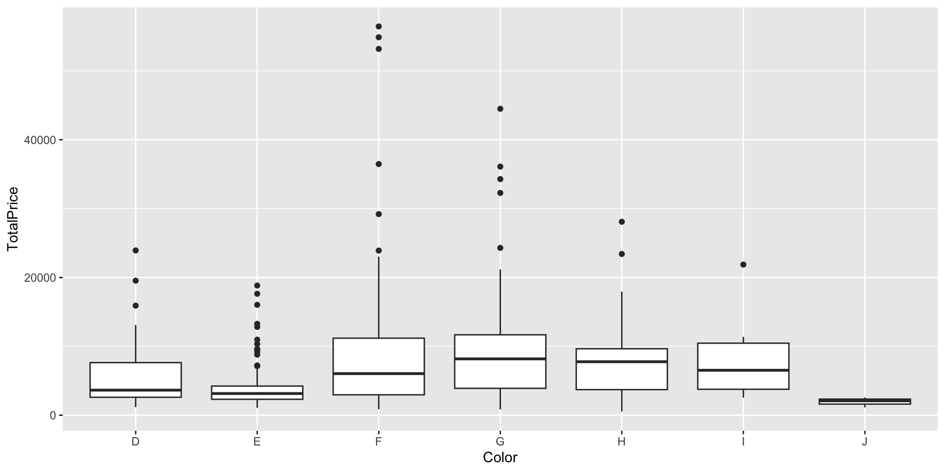
Transformations: Example
Diamonds %>%
  group_by(Color) %>%
  summarise(n = n(),
            m = mean(TotalPrice, na.rm = TRUE),
            sd = sd(TotalPrice, na.rm = TRUE))
# A tibble: 7 × 4
Color n m sd
<fct> <int> <dbl> <dbl>
1 D 52 5569. 4764.
2 E 82 4359. 3696.
3 F 87 9160. 10937.
4 G 86 9559. 7993.
5 H 29 8669. 6379.
6 I 12 7640. 5461.
7 J 3 1936. 737.[1] 14.86005Transformations: Example
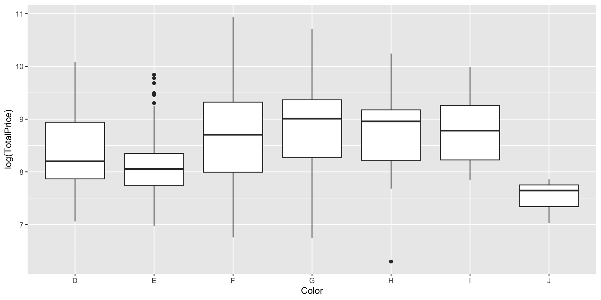
Log is not the only transformation!!
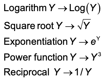
Common transformations
For the response (Y)…
When to use log transformation:
Look for:
- Distribution of response is skewed towards high end.
- The responses in one group (or more) range over two or more orders of magnitude.
- Variability (e.g., standard deviation) varies considerably across groups, especially when the spread is positively correlated with the mean.
When to NOT use a log transformation:
- When it doesn’t help
- When there is a better transformation to use
See page 236 Diagnostic Plot for Equalizing Spreads and example 5.21 for a general tool for finding an appropriate transformation.
How to transform
We can do the transformation directly in the visualization code:
OR, we can create a new variable in the dataset
Try it for the Hawks!
Let’s transformation the Weight variable to help the heterogeneity of variance issues for y = Weight and x = Species
- Check the S assumption on the raw data
- Transform: Use the following power function for your transformation: \(y^{0.43}\)
- Check the S assumption again on the transformed data
- Using the transformed data, create boxplots, run the ANOVA, and write a sentence interpretation of your ANOVA results.
Answer code
Hawks %>%
  group_by(Species) %>%
  summarise(m = mean(Weight, na.rm = TRUE),
            sd = sd(Weight, na.rm = TRUE))

189.21/80.65 #check S assumption

Hawks <- Hawks %>%
  mutate(Weight_new = (Weight)^.43) #transform

Hawks %>%
  group_by(Species) %>%
  summarise(m = mean(Weight_new, na.rm = TRUE),
            sd = sd(Weight_new, na.rm = TRUE))

2.19/1.43 # check S assumption with transformed data

ggplot(Hawks, aes(x = Species, y = Weight_new)) +
  geom_boxplot()

mod <- lm(Weight_new ~ Species, data = Hawks) #fitting anova model
anova(mod)
Mini Project Time
Mini Project 1
See Mini Project 1 instructions