# A tibble: 32 × 6
       X     Y     Z     W color    id
   <dbl> <dbl> <dbl> <dbl> <chr> <int>
 1   5.8   6      10     9 black     1
 2   5.6   6      10     9 black     2
 3   5.6   6      10     9 black     3
 4   3.8   4.5     4     2 white     4
 5   3.8   5       4     1 white     5
 6   5.4   6       8     8 black     6
 7   6     6      10    10 black     7
 8   3.5   4.5     3     2 white     8
 9   5.3   6       7     7 black     9
10   5.5   6       7     7 black    10
# ℹ 22 more rowsSampling Distributions
IMS, Ch. 12
2026-03-09
View distribution of r.v.’s
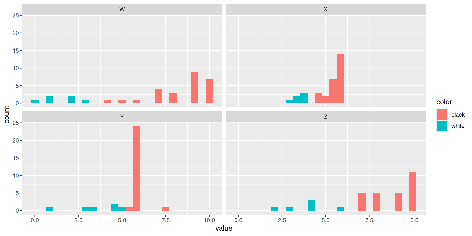
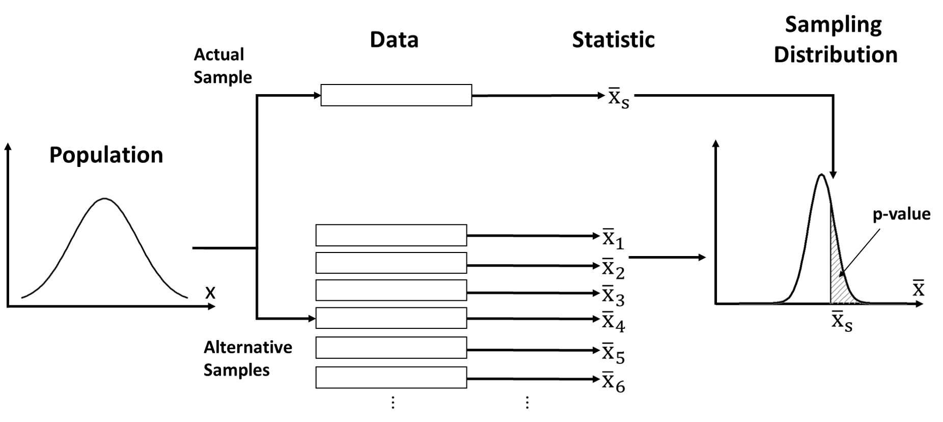
Sampling distribution
What if we resample from our sample?
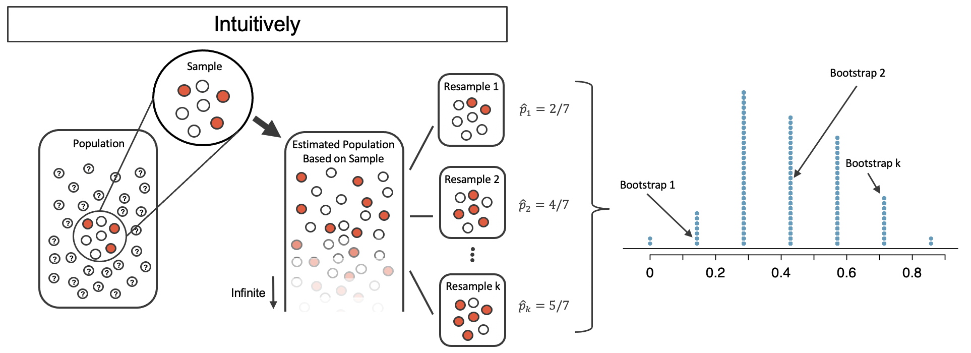
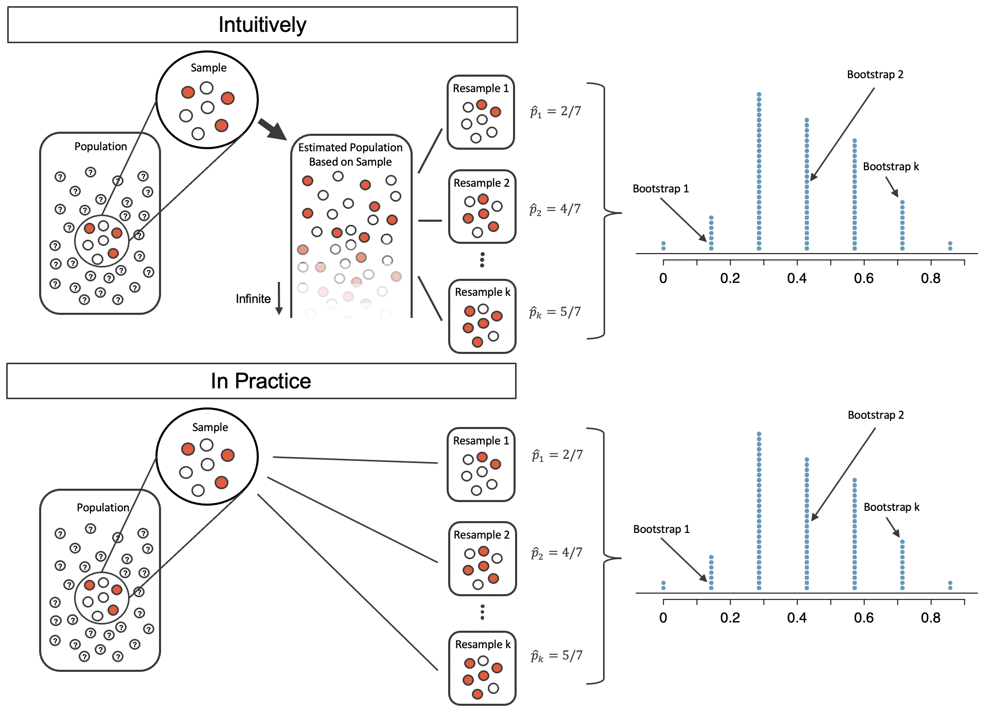
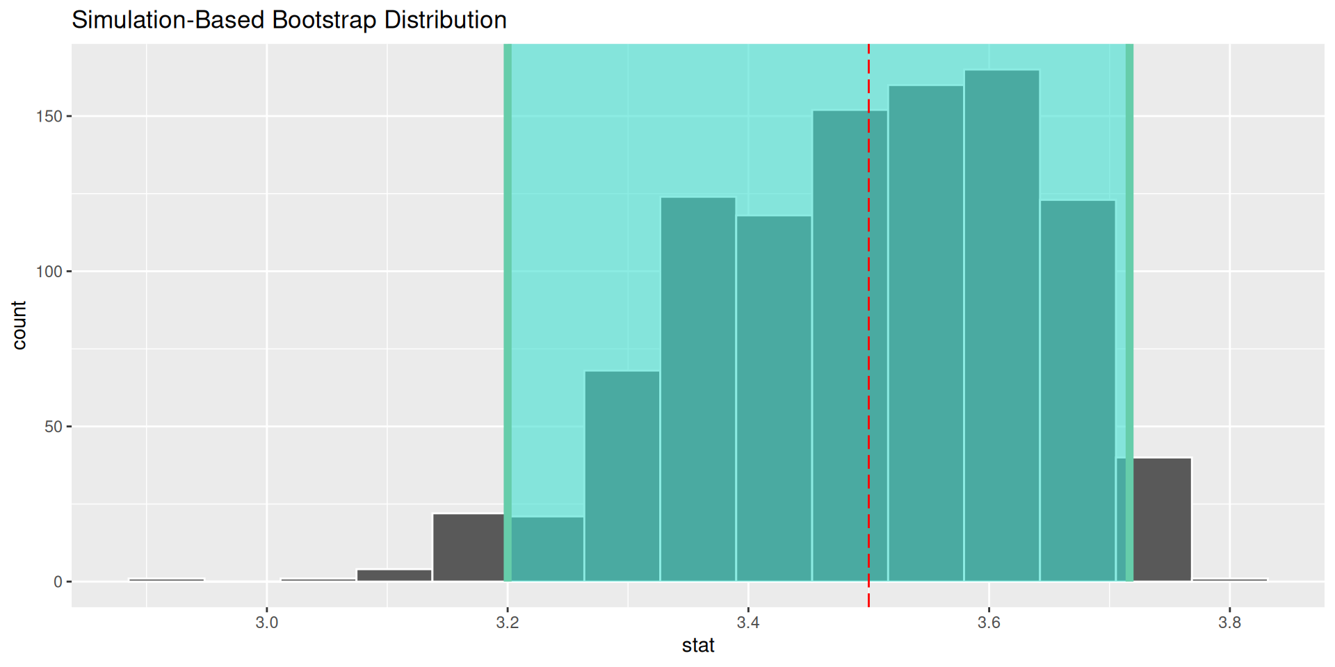
The bootstrap
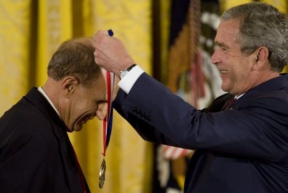
Developed by Brad Efron in 1979
- National Medal of Science (2005)
Resample from your sample with replacement!
Bootstrap distribution is similar to sampling distribution
The bootstrap distribution