Conditional Probability

OI, Ch. 3

Prof Randi Garcia

2026-02-27

Probability Worksheet

Probability Simulation

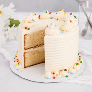
Suppose you have three two-layer cakes:

• one is vanilla on both layers
• one is chocolate on both layers
• one is vanilla on one layer and chocolate on the other

cake 1

cake 2

cake 3

Figure 1

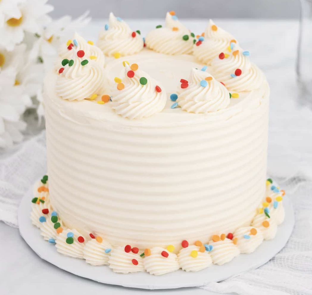
Probability Simulation

You cut the top layer and peek inside. It’s vanilla!

Q. What is the probability that when you cut through the bottom layer, that layer will also be vanilla?

Simulation

menu <- data.frame(
  layer_one = c("V", "V", "C"), 
  other_layer = c("V", "C", "C")
  )
menu

  layer_one other_layer
1         V           V
2         V           C
3         C           C

Simulation

library(tidyverse)
n <- 1000000
sim <- menu |>
  sample_n(size = n, replace = TRUE) |>
  mutate(
    cake_order = sample(c("layer_one_top", "other_layer_top"), 
                        size = n, 
                        replace = TRUE),
    peek = ifelse(cake_order == "layer_one_top", 
                  as.character(layer_one), 
                  as.character(other_layer)),
    full_cut = ifelse(cake_order == "layer_one_top", 
                      as.character(other_layer), 
                      as.character(layer_one))
    )

Simulation

sim |>
  head(10)

   layer_one other_layer      cake_order peek full_cut
1          V           V other_layer_top    V        V
2          V           V other_layer_top    V        V
3          C           C   layer_one_top    C        C
4          V           C other_layer_top    C        V
5          C           C other_layer_top    C        C
6          V           V other_layer_top    V        V
7          V           V other_layer_top    V        V
8          C           C   layer_one_top    C        C
9          C           C other_layer_top    C        C
10         V           C other_layer_top    C        V

Results

sim %>%
  filter(peek == "V") %>%
  summarize(
    peek_vanilla = n(), 
    full_cut_vanilla = sum(full_cut == "V")
    ) |>
  mutate(
    peek_vanilla_pct = peek_vanilla / n, 
    full_cut_pct = full_cut_vanilla / peek_vanilla
    )

  peek_vanilla full_cut_vanilla peek_vanilla_pct full_cut_pct
1       500148           333709         0.500148    0.6672205

Conditional Probability

Properties

Let \(A, B\) be two events. Then:

• Law of Total Probability: \[ \mathrm{P}(A) = \mathrm{P}(A \text{ and } B) + \mathrm{P}(A \text{ and } B^c) \]
• Definition of Conditional Probability: \[ \mathrm{P}(A |B) = \frac{\mathrm{P}(A \text{ and } B)}{\mathrm{P}(B)} \]

Picture

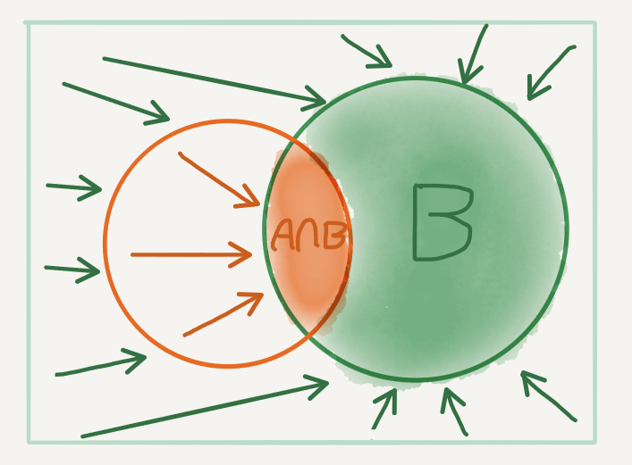
• Caveat: It is never safe to assume that \(\mathrm{P}(A|B) = \mathrm{P}(B|A)\)!
• What happens when event A is very unlikely to occur?

Independence

\(A\) and \(B\) are independent if and only if:

• \(\mathrm{P}(A | B) = \mathrm{P}(A)\), and
• \(\mathrm{P}(B | A) = \mathrm{P}(B)\)

Note that this implies \(\mathrm{P}(A \text{ and } B) = \mathrm{P}(A) \times \mathrm{P}(B)\)

• Do not confuse independence with disjointness! Two events that are disjoint are not independent, since if one happens, you know the other one doesn’t happen!
• General multiplication rule: \[ \mathrm{P}(A|B) \times \mathrm{P}(B) = \mathrm{P}(A \text{ and } B) = \mathrm{P}(B|A)\times \mathrm{P}(A) \]

Bayes’ Rule

\[ \mathrm{P}(A|B) = \frac{\mathrm{P}(B|A) \times \mathrm{P}(A)}{\mathrm{P}(B)} \]

• Translate \(\mathrm{P}(A|B)\) into \(\mathrm{P}(B|A)\)
• Foundation for Bayesian statistics

Example: Hair Whorls and Handedness

When my daughter was a baby I noticed her hair whorl swirled counterclockwise (CCW). It turns out that CCW whorls are less common than clockwise (CW) whorls. Further, whorl direction and handedness have been found to be associated (Klar, 2003)! I wondered, given that my baby had a CCW whorl, what was the chance she’d be left-handed?

Example: Hair Whorls and Handedness

• Event B is counterclockwise hair whorl, \(\mathrm{P}(B) = .23\)
• Event A is left handedness, \(\mathrm{P}(A) = .12\)
• 45% of left handed people were found to have CCW hair whorls, \(\mathrm{P}(B|A) = .45\)

So, given that my baby had a CCW whorl, what was the chance she’d be left-handed? We need \(\mathrm{P}(A|B)\)

\[ \mathrm{P}(A|B) = \frac{\mathrm{P}(B|A) \times \mathrm{P}(A)}{\mathrm{P}(B)} = \frac{.45 \times .12}{.23} = .235 \]

Contingency tables

• Joint probabilities in the middle of the table

library(openintro)
yawn |>
  group_by(group, result) |>
  count() |>
  pivot_wider(names_from = result, values_from = n)

# A tibble: 2 × 3
# Groups:   group [2]
  group `not yawn`  yawn
  <fct>      <int> <int>
1 ctrl          12     4
2 trmt          24    10

Tables with margins

• marginal probabilities on the outside

library(janitor)
yawn |>
  tabyl(group, result) |>
  adorn_totals(c("row", "col"))

 group not yawn yawn Total
  ctrl       12    4    16
  trmt       24   10    34
 Total       36   14    50