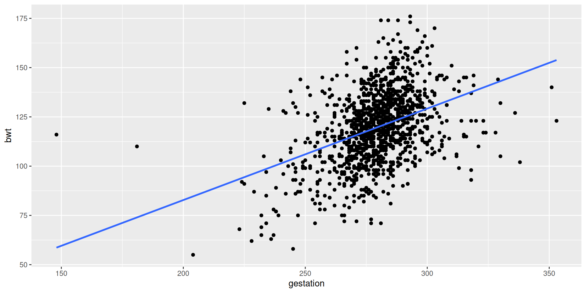
(Intercept)   gestation
-10.0641842 0.4642626 Simple linear regression
IMS, Ch. 7
Prof Randi Garcia
2026-02-09
Warmup
Warmup 1
An article reported that there was a 0.42 correlation between alcohol consumption and income among adults with a four-year college degree.
Is it reasonable to conclude that increasing one’s alcohol consumption will increase one’s income? Explain why or why not.
Warmup 2
A college newspaper interviews a psychologist about student ratings of the teaching of faculty members.
The psychologist says, “The evidence indicates that the correlation between the research productivity and teaching rating of faculty members is close to zero.”
The paper reports this as “Prof. McDaniel said that good researchers tend to be poor teachers, and vice versa.”
Explain why the paper’s report is wrong.
Write a statement in plain language (don’t use the word correlation) to explain the psychologist’s meaning.
Simple linear regression
Regression
Goal: understand changes in a numerical response variable in terms of a numerical explanatory variable.
A simple linear regression model for \(y\) in terms of \(x\) takes the form: \[ y_i = \beta_0 + \beta_1 \cdot x_i + \epsilon_i \,, \text{ for } i=1,\ldots,n \]
- \(y_i\) and \(x_i\) for \(i = 1, \ldots, n\) are the observations
- \(\beta_0\) is the intercept
- \(\beta_1\) is the slope coefficient
- \(\epsilon_i\)’s are the errors, or noise
Computing
- Use
lm()to fit the model - Use
coef()on the regression object to get the coefficients
View model in the data space
- Use
geom_smooth(method = "lm")to show on a plot
Properties of SLR models
Recall: Parameter vs. Statistic
- Only one regression line that fits the data best using a least squares criteria
- ordinary least squares regression line is unique
- The true values of the unknown parameters \(\beta_0\) and \(\beta_1\) are estimated by \(b_0\) and \(b_1\)
- (or if you prefer, \(\hat{\beta_0}\) and \(\hat{\beta_1}\))
- The fitted values are given by \[ \hat{y}_i = b_0 + b_1 \cdot x_i \]
Residuals
The model (almost) never fits perfectly
What is left over are the residuals (\(e_i = y_i - \hat{y_i}\))
Many of the assumptions we’ll make later involve the residuals
Residual analysis is important! (…more later)
Example: RailTrail
The Pioneer Valley Planning Commission (PVPC) collected data north of Chestnut Street in Florence, MA for ninety days from April 5, 2005 to November 15, 2005. Data collectors set up a laser sensor, with breaks in the laser beam recording when a rail-trail user passed the data collection station. The data is captured in the RailTrail data set.
Rows: 90
Columns: 11
$ hightemp   <int> 83, 73, 74, 95, 44, 69, 66, 66, 80, 79, 78, 65, 41, 59, 50,…
$ lowtemp    <int> 50, 49, 52, 61, 52, 54, 39, 38, 55, 45, 55, 48, 49, 35, 35,…
$ avgtemp    <dbl> 66.5, 61.0, 63.0, 78.0, 48.0, 61.5, 52.5, 52.0, 67.5, 62.0,…
$ spring     <int> 0, 0, 1, 0, 1, 1, 1, 1, 0, 0, 0, 1, 1, 0, 0, 1, 0, 1, 1, 0,…
$ summer     <int> 1, 1, 0, 1, 0, 0, 0, 0, 1, 1, 1, 0, 0, 0, 0, 0, 1, 0, 0, 0,…
$ fall       <int> 0, 0, 0, 0, 0, 0, 0, 0, 0, 0, 0, 0, 0, 1, 1, 0, 0, 0, 0, 1,…
$ cloudcover <dbl> 7.6, 6.3, 7.5, 2.6, 10.0, 6.6, 2.4, 0.0, 3.8, 4.1, 8.5, 7.2…
$ precip     <dbl> 0.00, 0.29, 0.32, 0.00, 0.14, 0.02, 0.00, 0.00, 0.00, 0.00,…
$ volume     <int> 501, 419, 397, 385, 200, 375, 417, 629, 533, 547, 432, 418,…
$ weekday    <lgl> TRUE, TRUE, TRUE, FALSE, TRUE, TRUE, TRUE, FALSE, FALSE, TR…
$ dayType    <chr> "weekday", "weekday", "weekday", "weekend", "weekday", "wee…
Your turn: RailTrail
- Create a scatterplot for the
volumein terms ofavgtemp - Describe the form, direction, and strength of the relationship
- Compute the correlation coefficient
- Use
geom_smooth()to view the model in the data space - Fit the linear regression model using
lm() - Interpret the coefficients for the
Interceptandavgtempterms
Model visualization
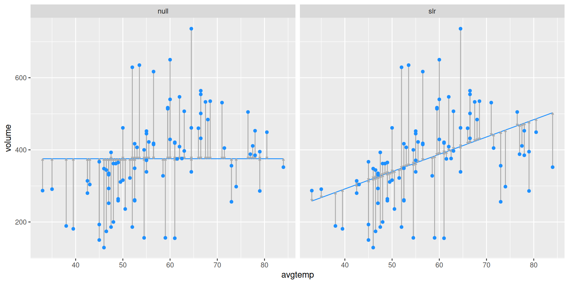
Compare the least squares regression line (right) with the null model (left).