Center, Shape, and Spread

IMS, Ch. 4–5

Prof Randi Garcia

2026-02-04

Warmup

Lurking Variables

For each of the following pairs of variables, a statistically significant positive relationship has been observed. Identify a potential lurking variable (omitted confounder) that might cause the spurious correlation.

  • The amount of ice cream sold in New England and the number of deaths by drowning
  • The salary of U.S. ministers and the price of vodka
  • The number of doctors in a region and the number of crimes committed in that region
  • The amount of coffee consumed and the prevalence of lung cancer

Summarizing distributions

  • Shape, Center, and Spread

Histogram

Summarize the shape of the distribution of one variable
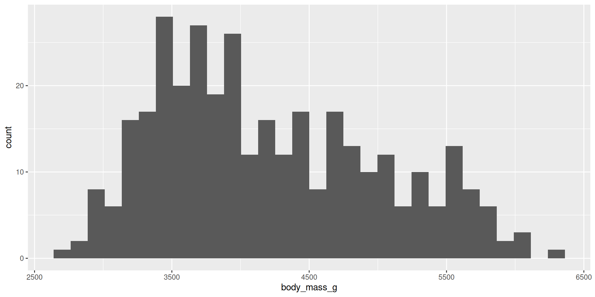
library(tidyverse)
library(palmerpenguins)
ggplot(data = penguins, aes(x = body_mass_g)) +
  geom_histogram()

Density plot

Summarize the shape of the distribution of one variable
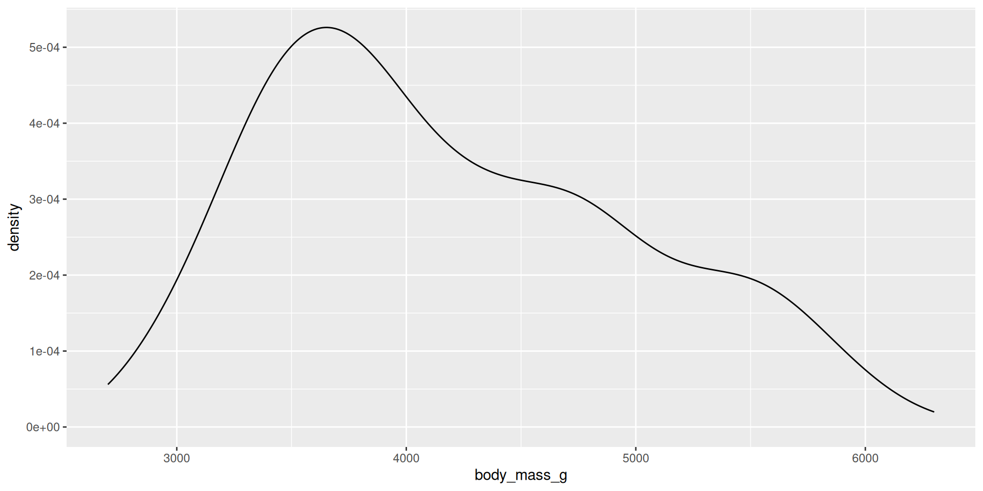
ggplot(data = penguins, aes(x = body_mass_g)) +
  geom_density()

Box plot

Summarize the shape of the distribution of one variable
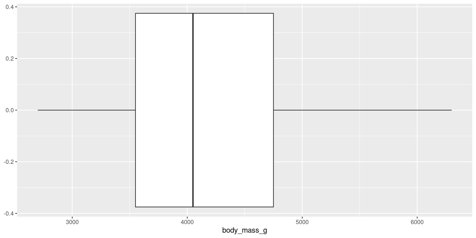
ggplot(data = penguins, aes(x = body_mass_g)) +
  geom_boxplot()

Your turn

  • Use a data graphic to summarize the distribution of the height variable in the starwars data frame.

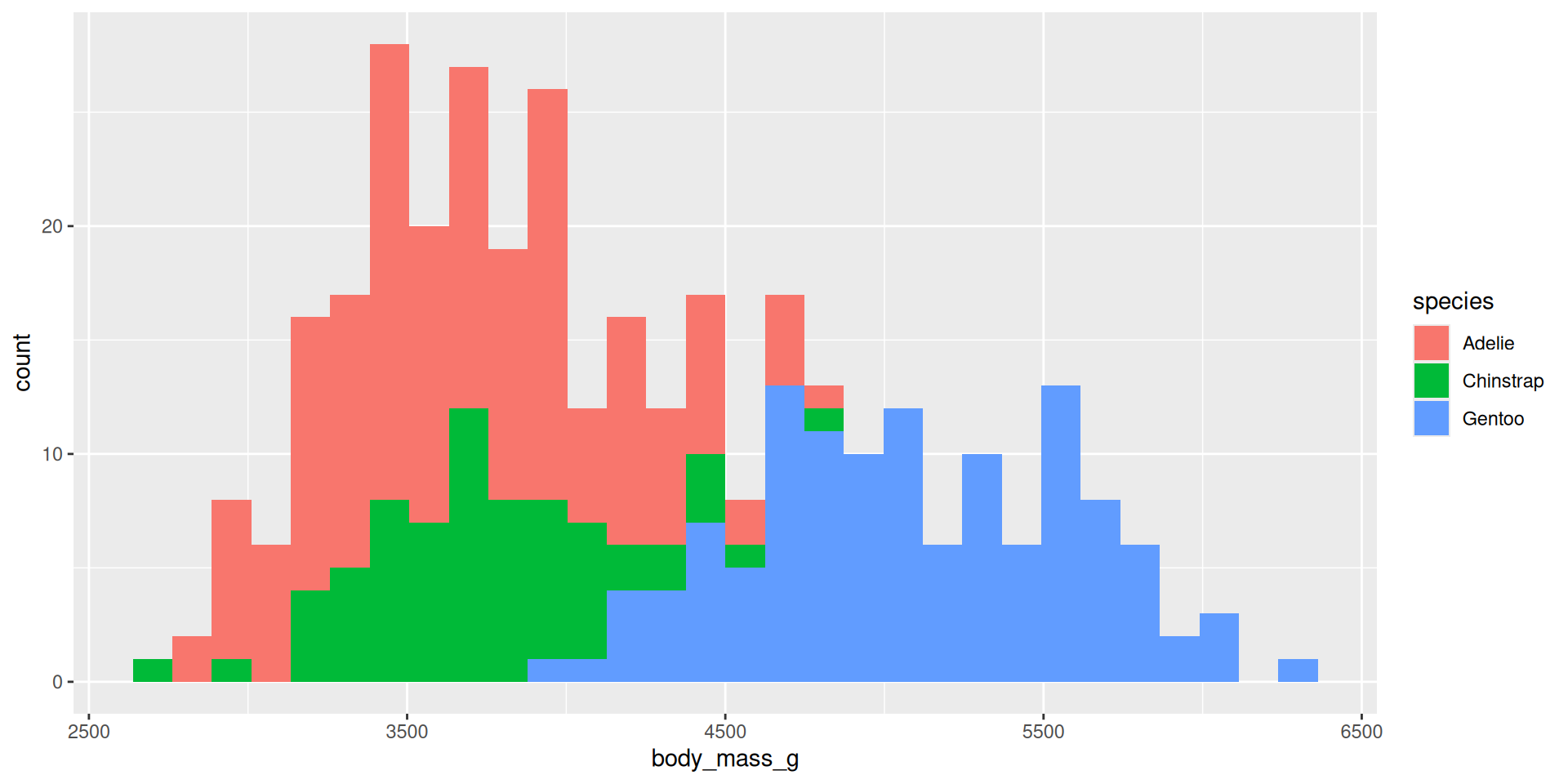
Histogram: two variables

ggplot(data = penguins, aes(x = body_mass_g, fill = species)) +
  geom_histogram()

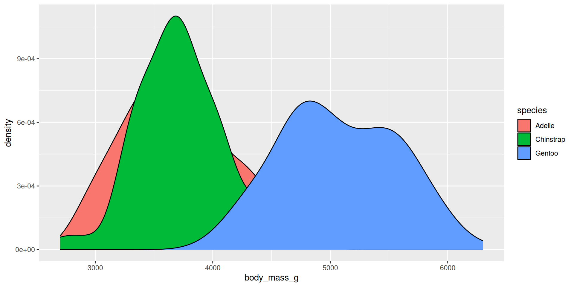
Density plot: two variables

ggplot(data = penguins, aes(x = body_mass_g, fill = species)) +
  geom_density()

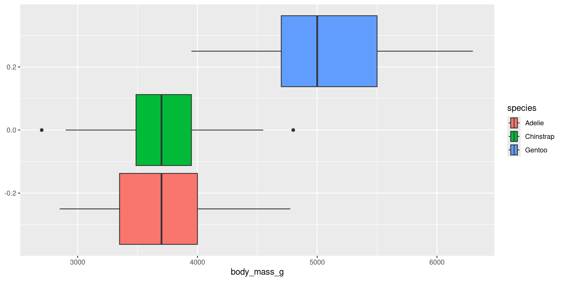
Boxplot: two variables

ggplot(data = penguins, aes(x = body_mass_g, fill = species)) +
  geom_boxplot()

Measures of center

  • mean: mean()
  • median: median()
penguins |>
  summarize(
    number_of_penguins = n(),
    mean_mass = mean(body_mass_g, na.rm = TRUE),
    median_mass = median(body_mass_g, na.rm = TRUE)
  )
# A tibble: 1 × 3
  number_of_penguins mean_mass median_mass
               <int>     <dbl>       <dbl>
1                344     4202.        4050

Measures of spread

  • standard deviation: sd()
  • variance: var()
  • range: range()
  • IQR: IQR()
penguins |>
  summarize(
    number_of_penguins = n(),
    sd_mass = sd(body_mass_g, na.rm = TRUE),
    var_mass = var(body_mass_g, na.rm = TRUE)
  )
# A tibble: 1 × 3
  number_of_penguins sd_mass var_mass
               <int>   <dbl>    <dbl>
1                344    802.  643131.

Your turn

  • Summarize the distribution of the height variable in the starwars data frame by computing:
    • the number of observations
    • the mean
    • the standard deviation

Thought Experiment

Consider the following two variables:

  1. The height of all adults in the United States
  2. The annual income of all working adults in the United States
  • Sketch a density plot for each distribution. What features does it have?
  • Is it symmetric? Is it normal? It is unimodal?
  • Summarize each distribution numerically. Which measures are most appropriate?

Challenge

Suppose that the government issued a tax rebate in the amount of $2000 to each American taxpayer.

  • How would the distribution of income change?
  • What would happen to your measures of center and spread?